Code
library(lattice)
library(latticeExtra)![]()

lattice and latticeExtra PackagesThe lattice package in R is a powerful system for creating Trellis graphics, which allow for multivariate data visualization through conditioning (splitting data into panels) and grouping (overlaying subgroups). It builds on the base R graphics but emphasizes high-level, elegant plots for statistical analysis. The latticeExtra package extends lattice with additional functions for more flexible and specialized plots, such as empirical CDFs, smoothed surfaces, and layered visualizations.
This tutorial assumes basic familiarity with R and data frames. We’ll use built-in datasets like Chem97 (from mlmRev), quakes, and singer (from latticeExtra). By the end, you’ll be able to create conditioned scatter plots, box plots, density estimates, and advanced overlays.
Install the packages from CRAN if you haven’t already:
install.packages(c("lattice", "latticeExtra"))Load them in your R session:
library(lattice)
library(latticeExtra)latticelattice provides high-level functions for common statistical graphics. Let’s start with simple examples using the Chem97 dataset (GCSE and A-level scores for UK students), is part of the {mlmRev} package.
xyplot()The xyplot() function creates scatter plots, ideal for two continuous variables.
library(mlmRev)Loading required package: lme4Loading required package: Matrixdata(Chem97)
# Basic scatter plot
xyplot(score ~ gcsecnt, data = Chem97,
main = "GCSE vs. A-level Scores",
xlab = "A-level Score", ylab = "GCSE Score")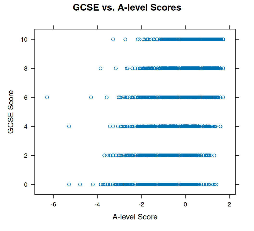
This produces a single panel scatter plot. To add grouping (e.g., by gender), use the groups argument:
xyplot(score ~ gcsecnt, data = Chem97,
       groups = gender,
       auto.key = list(title = "Gender", columns = 2),
       main = "GCSE vs. A-level Scores by Gender")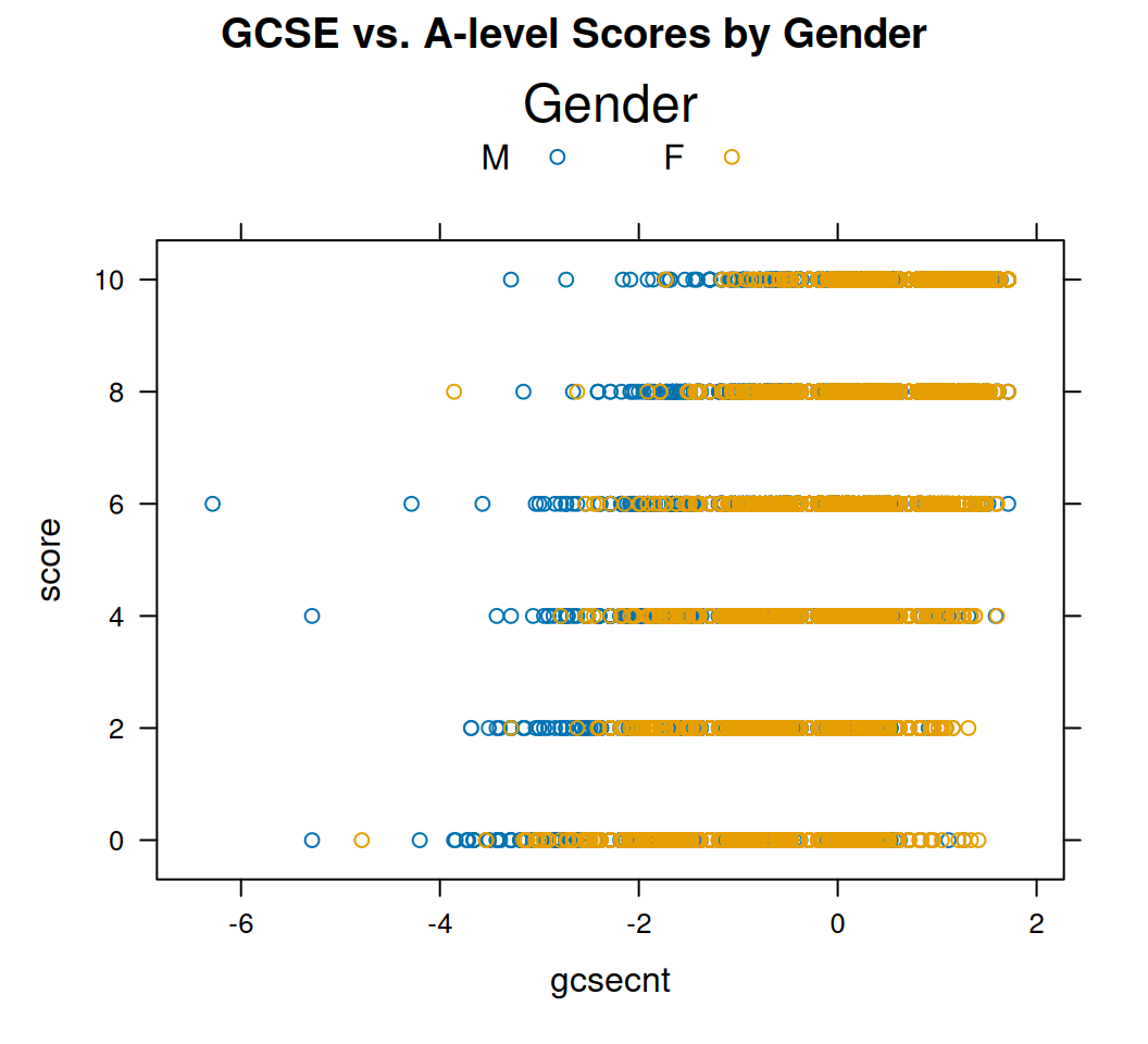
The auto.key adds a legend automatically.
histogram()For univariate distributions:
# Simple histogram
histogram(~ score, data = Chem97,
          main = "Distribution of GCSE Scores")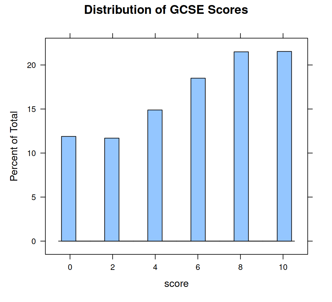
bwplot()Compare distributions across categories:
bwplot(gcsescore ~ factor(score), data = Chem97,
       main = "GCSE Scores by A-level Band",
       xlab = "A-level Band")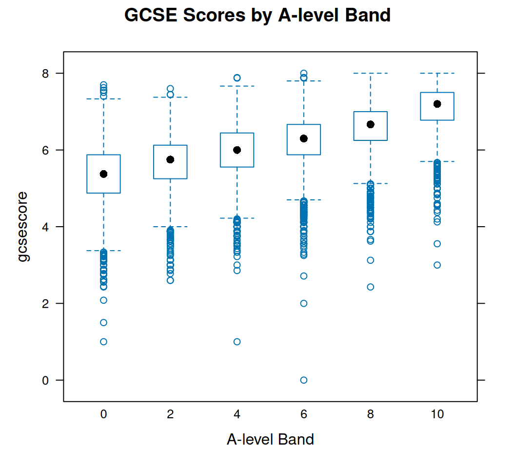
latticeConditioning splits the plot into panels using | condition in the formula, great for multivariate comparisons. Grouping overlays lines or points within panels.
densityplot()Kernel density estimates, conditioned by a factor:
densityplot(~ gcsescore | factor(score), data = Chem97,
            groups = gender,
            plot.points = FALSE,  # Omit raw points for clarity
            auto.key = list(title = "Gender", columns = 2),
            main = "Density of GCSE Scores by A-level Band and Gender")
This creates a multi-panel plot (one per A-level band) with overlaid densities for males and females.
qqmath()Check normality, grouped and conditioned:
qqmath(~ gcsescore | factor(score), data = Chem97,
       groups = gender,
       f.value = ppoints(100),  # Theoretical quantiles
       auto.key = list(title = "Gender"),
       type = c("p", "g"),  # Points and grid lines
       aspect = "xy",  # Equal aspect ratio
       main = "Q-Q Plots of GCSE Scores")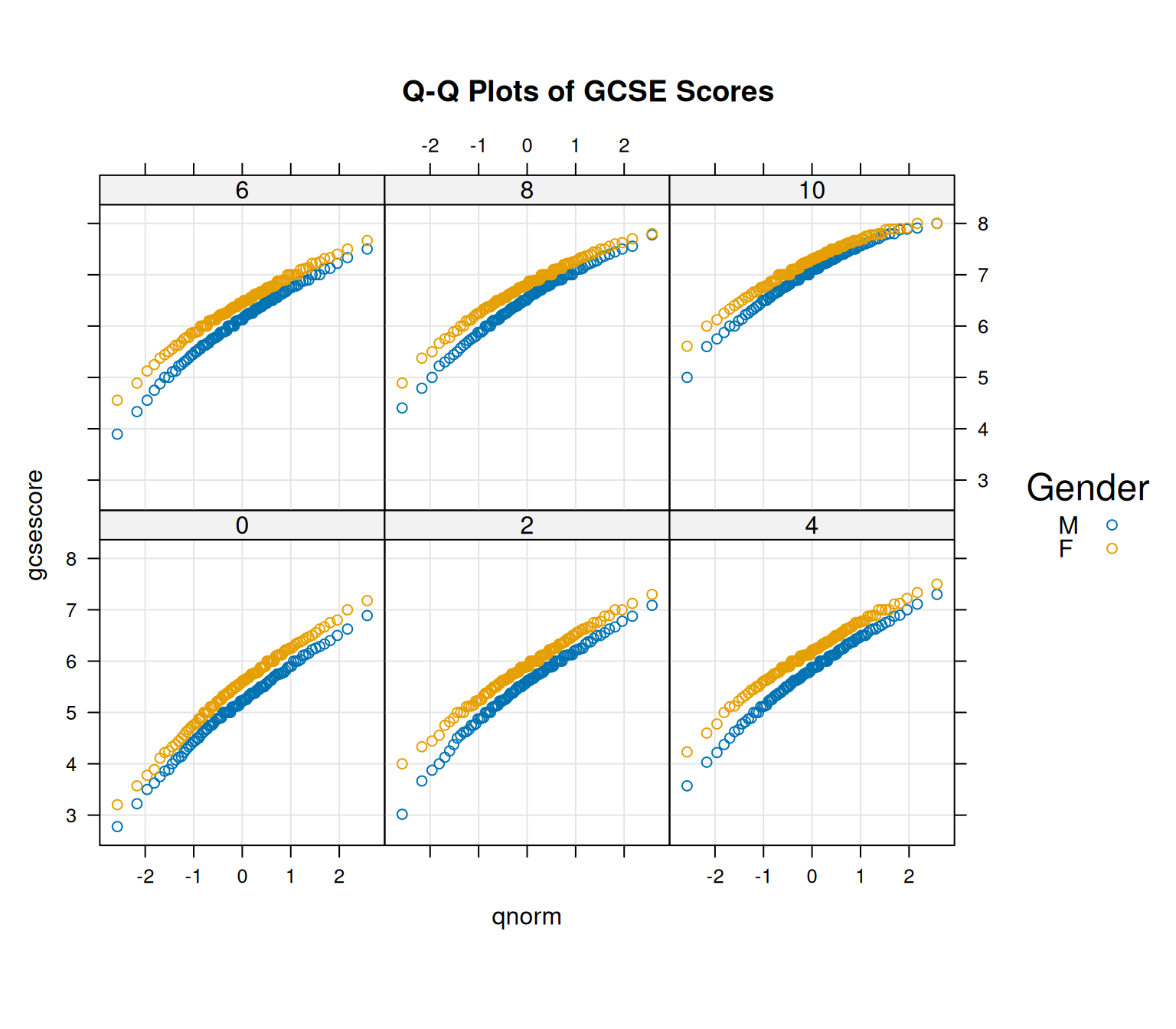
qq()Compare two groups:
qq(gender ~ gcsescore | factor(score), data = Chem97,
   f.value = ppoints(100),
   type = c("p", "g"),
   aspect = 1,
   main = "Comparing Male vs. Female GCSE Scores by Band")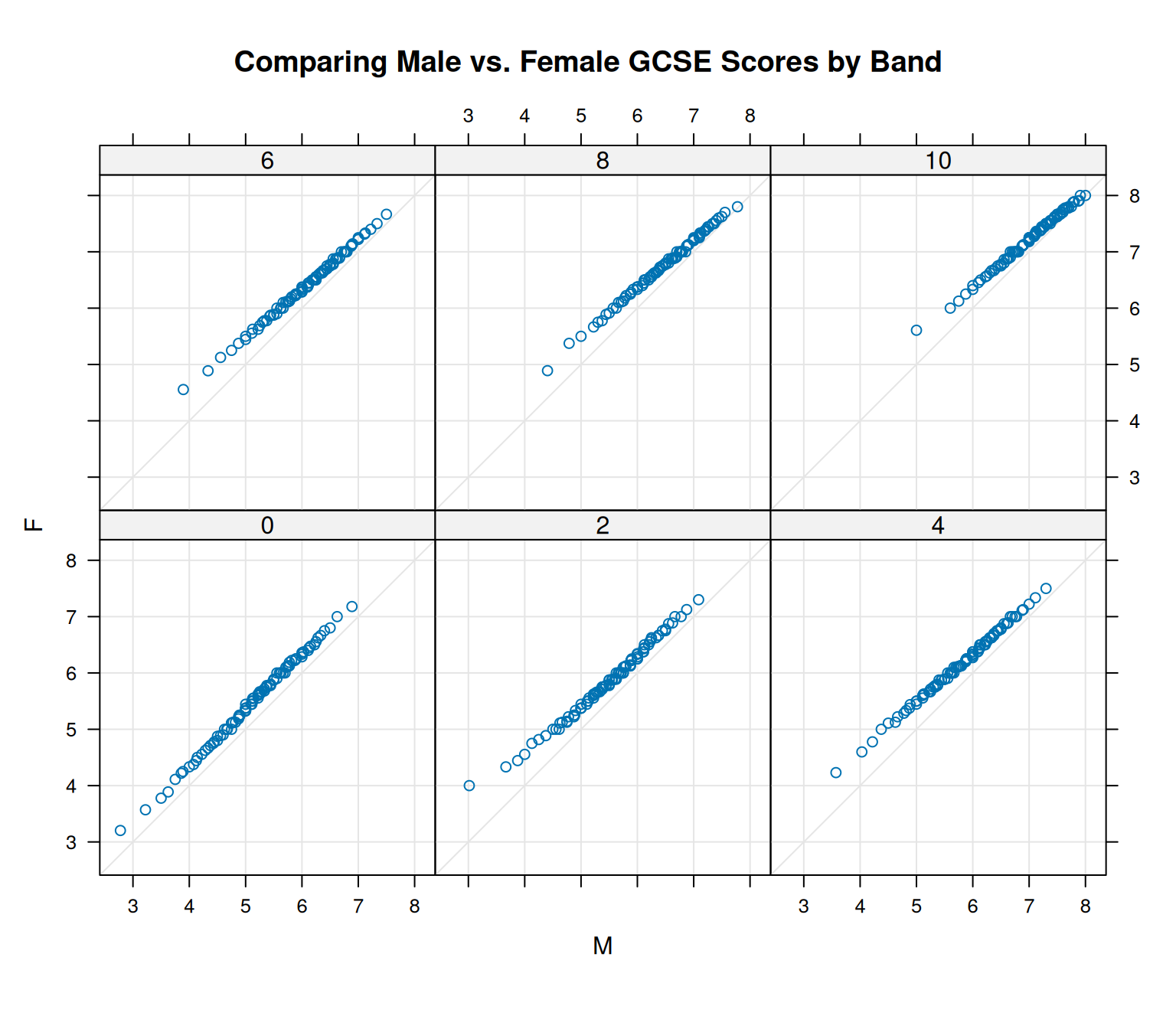
stripplot()For jittered 1D scatters (like a conditioned stripchart):
stripplot(depth ~ factor(mag), data = quakes,
          jitter.data = TRUE,
          alpha = 0.6,  # Transparency
          main = "Earthquake Depth by Magnitude",
          xlab = "Magnitude (Richter)", ylab = "Depth (km)")
This uses the quakes dataset for a quick multivariate view.
latticeExtralatticeExtra adds utilities for layering, scaling, and specialized plots. It integrates seamlessly with lattice objects.
ecdfplot()Non-parametric cumulative distributions:
ecdfplot(~ height | voice.part, data = singer,
         main = "Empirical CDF of Singer Heights by Voice Part")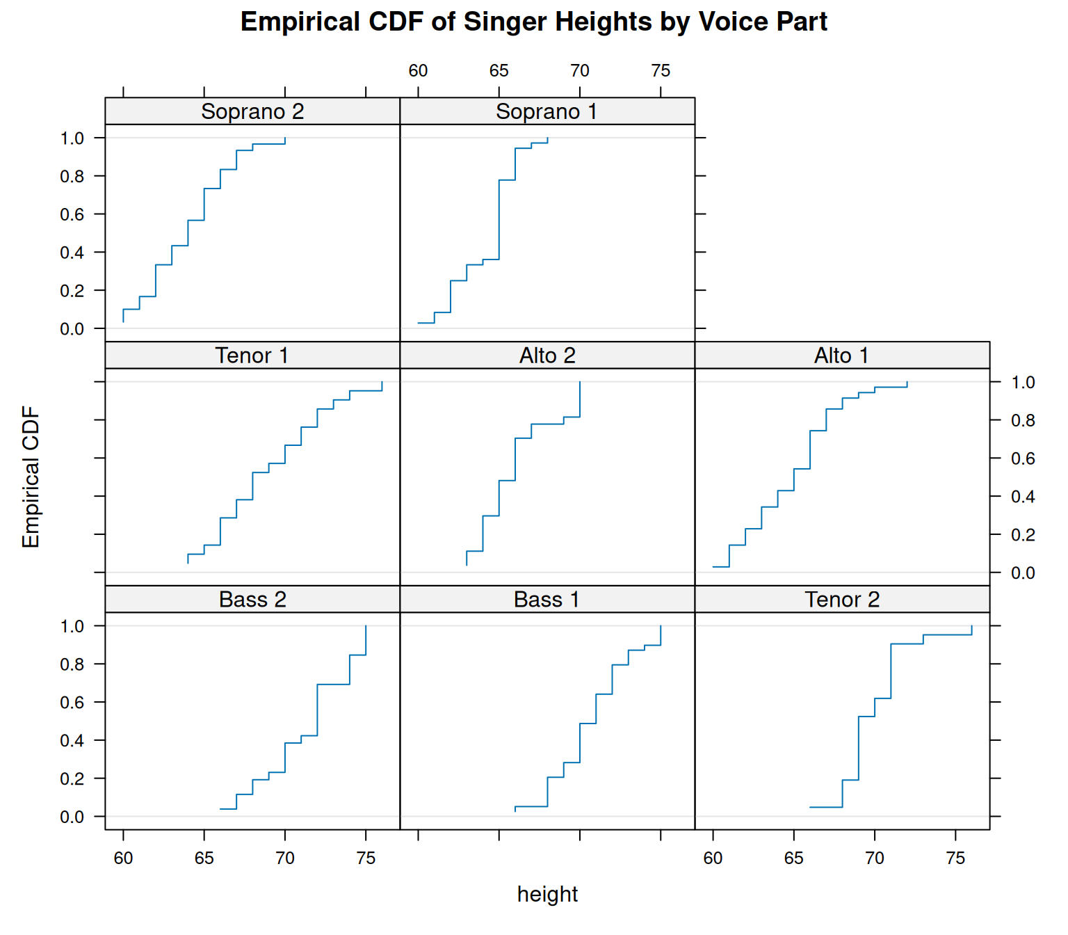
Using the singer dataset, this conditions on voice parts (e.g., Tenor, Bass).
layer()Add custom layers to existing plots, like smoothers:
p <- xyplot(lat ~ long, data = quakes,
            main = "Earthquake Locations with Density Overlay",
            xlab = "Longitude", ylab = "Latitude",
            alpha = 0.5, pch = 19)
p + layer(panel.2dsmoother(...), style = 1)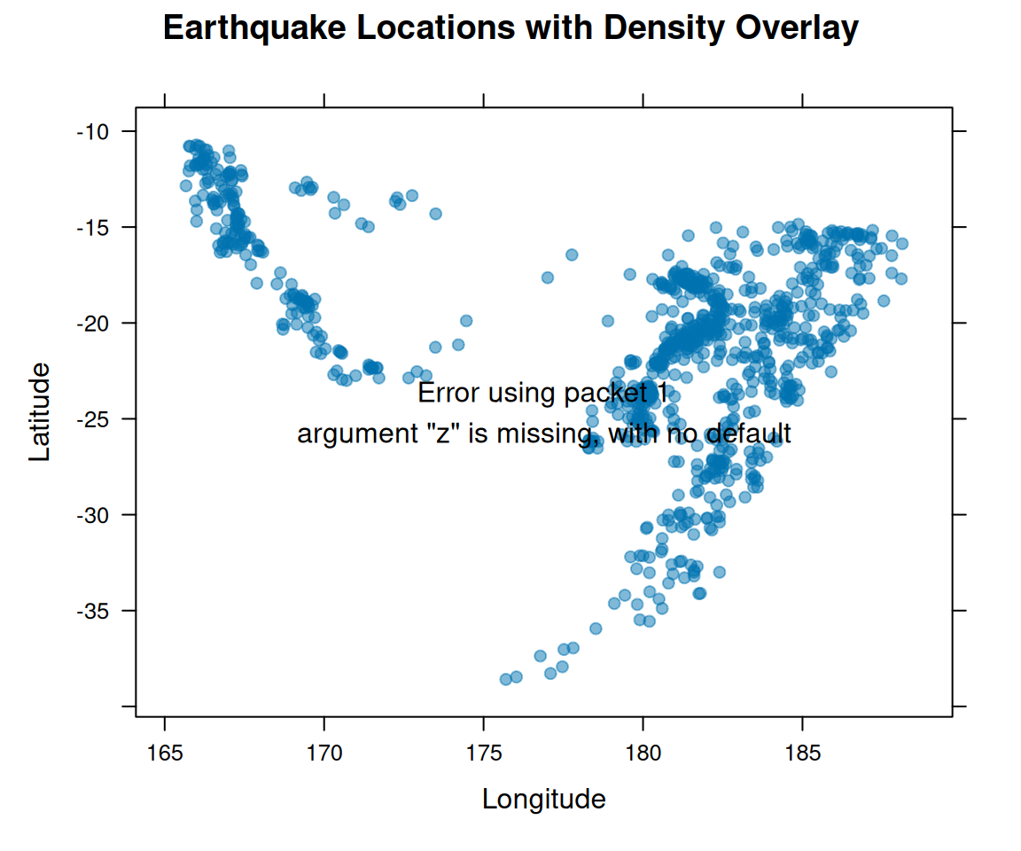
For quantile regression:
library(quantreg) # Required for quantile regressionLoading required package: SparseM
Attaching package: 'SparseM'The following object is masked from 'package:Matrix':
detdata(quakes) # Load quakes dataset
xyplot(depth ~ mag, data = quakes,
main = "Quantile Regression of Earthquake Depth vs. Magnitude",
xlab = "Magnitude (Richter)", ylab = "Depth (km)",
alpha = 0.5, pch = 19) +
layer(panel.quantile(x, y, tau = c(0.5, 0.9, 0.1), superpose = TRUE)) +
layer(auto.key = list(text = c("50%", "90%", "10%"), points = FALSE, lines = TRUE))
doubleYScale()Plot two series with different scales:
# Create two xyplot objects
p1 <- xyplot(depth ~ mag, data = quakes, type = "l", col = "red",
             main = "Depth and Stations vs. Magnitude",
             xlab = "Magnitude (Richter)", ylab = "Depth (km)")
p2 <- xyplot(stations ~ mag, data = quakes, type = "l", col = "blue",
             xlab = "Magnitude (Richter)", ylab = "Stations")

# Combine with doubleYScale
doubleYScale(p1, p2, use.style = TRUE,
             auto.key = list(text = c("Depth", "Stations"), lines = TRUE, points = FALSE))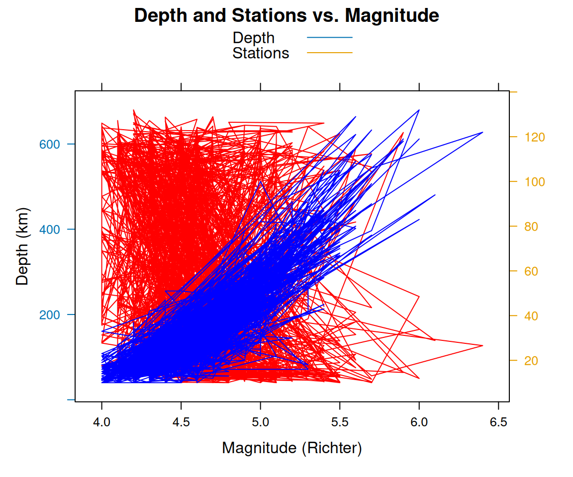
Combine levelplot() from lattice with latticeExtra panels for smoothed heatmaps. For three numeric variables (x, y, z), plot points and add a 2D smoother:
# Assuming data with x, y, z columns
levelplot(depth ~ long * lat, data = quakes,
          main = "Smoothed Heatmap of Earthquake Depth near Tonga Trench",
          xlab = "Longitude", ylab = "Latitude",
          col.regions = colorRampPalette(c("blue", "white", "red"))(100),
          panel = function(...) {
            panel.levelplot.points(..., pch = 19, alpha = 0.5)  # Add points
            panel.2dsmoother(...)  # Add smoothed surface
          })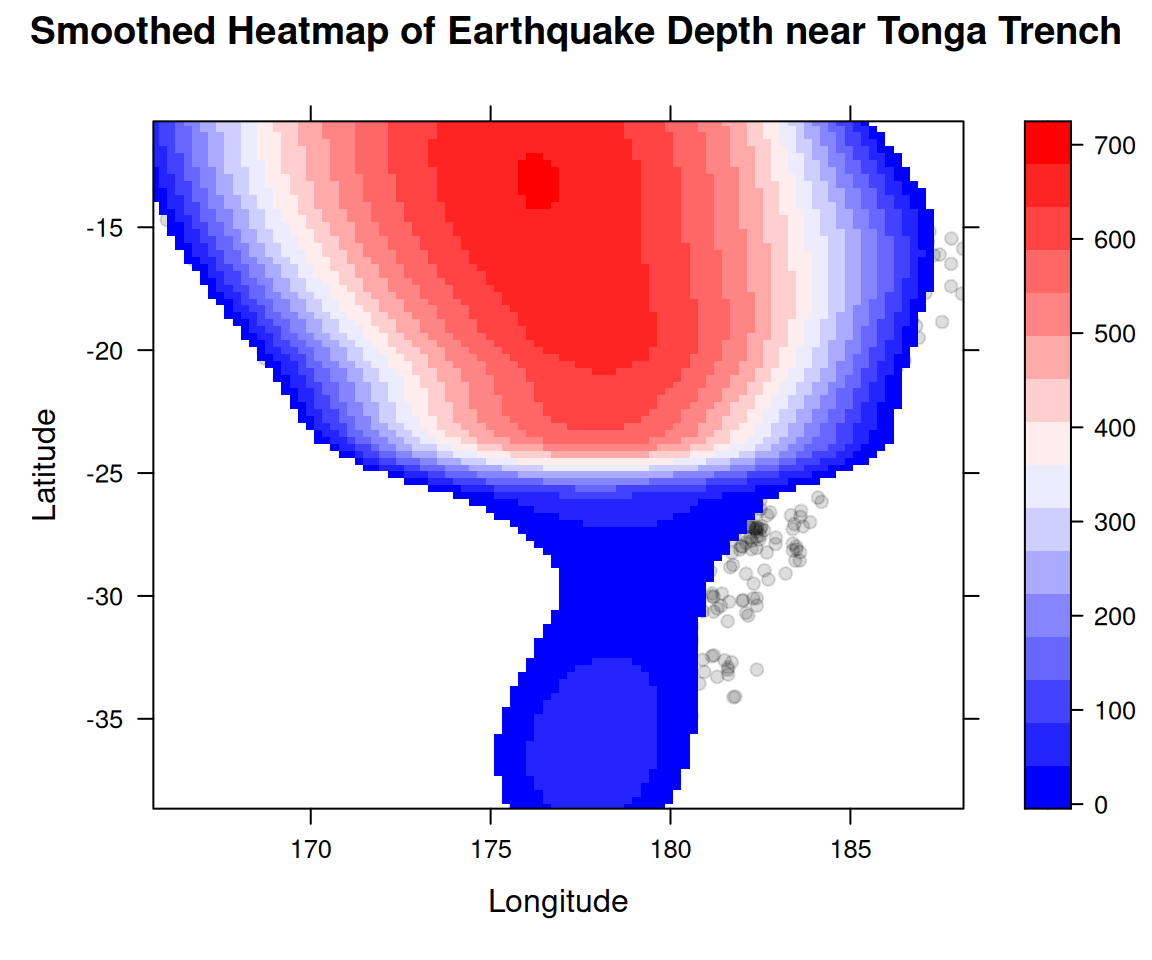
This visualizes individual points alongside a smoothed surface, blending scatter and heatmap elements.
c.trellis()Combine multiple Trellis objects:
library(gridExtra)
# Create histogram and density plot
p1 <- histogram(~ mag, data = quakes,
                main = "Histogram of Earthquake Magnitudes",
                xlab = "Magnitude (Richter)")
p2 <- densityplot(~ mag, data = quakes,
                 main = "Density Plot of Earthquake Magnitudes",
                 xlab = "Magnitude (Richter)")

# Combine plots using grid.arrange
grid.arrange(p1, p2, nrow = 2, top = "Earthquake Magnitude Distributions")
Customize appearance with themes from latticeExtra:
# Apply a ggplot2-like theme
trellis.par.set(ggplot2like())
# Or Economist style
trellis.par.set(theEconomist.theme())
For panel-specific tweaks, use panel functions like panel.ablineq() to add labeled lines.
as.data.frame.table().layout to control arrangement, e.g., layout = c(2, 3)).alpha for transparency.print() explicitly if needed in scripts.?xyplot for details, or Deepayan Sarkar’s book Lattice: Multivariate Data Visualization with R.This tutorial demonstrated the lattice and latticeExtra packages in R using the quakes dataset (1000 seismic events near the Tonga Trench). Key visualizations included scatter plots, histograms, density plots, box plots, quantile regression, dual y-axis plots, smoothed heatmaps, and combined plots using grid.arrange() from gridExtra. The examples showcased conditioning, grouping, and customization for multivariate analysis, with fixes for errors like c.trellis() and variable referencing.
lattice excels in creating clear, multivariate Trellis graphics, surpassing base R for complex datasets like quakes. latticeExtra enhances it with advanced features like quantile regression and smoothed surfaces. While powerful, it requires learning the formula interface and may need subsampling for large datasets. It complements ggplot2 and plotly for static, high-quality visualizations.
lattice reference manual and vignettes. CRAN