Code
packages <- c(
          'tidyverse'
) ![]()

readr offers a fast and user-friendly method of reading rectangular-shaped data from delimited files, including comma-separated values (CSV) and tab-separated values (TSV). Its design is intended to parse various data types encountered in real-world scenarios, and it provides a comprehensive problem report that informs you when parsing leads to unexpected outcomes or when the data is not in the expected format. This package is part of the tidyverse collection of packages, which are designed to work together seamlessly and share a common design philosophy.

The easiest way to get {readr} is to install the tidyverse. The tidyverse is a collection of R packages designed for data science. It includes several packages that work well together to facilitate data manipulation, visualization, and analysis in a consistent and coherent manner. Some key packages within the tidyverse include {ggplot2} for plotting, {dplyr} for data manipulation, {tidyr} for data tidying, {readr} for data import, and more. The tidyverse is designed to make data science easier and more efficient by providing a set of tools that share a common design philosophy and grammar. This allows users to work with data in a more intuitive and streamlined way, reducing the need for repetitive coding and making it easier to create reproducible analyses.
![]()
The core tidyverse includes the packages that you’re likely to use in everyday data analyses. As of tidyverse 1.3.0, the following packages are included in the core tidyverse:
As well as {readr}, for reading flat files, the {tidyverse} package installs a number of other packages for reading data:
DBI for relational databases. You’ll need to pair DBI with a database specific backends like RSQLite, RMariaDB, RPostgres, or odbc. Learn more at https://db.rstudio.com.
haven for SPSS, Stata, and SAS data.
httr for web APIs.
readxl for .xls and .xlsx sheets.
googlesheets4 for Google Sheets via the Sheets API v4.
googledrive for Google Drive files.
rvest for web scraping.
sonlite for JSON. (Maintained by Jeroen Ooms.)
xml2 for XML
packages <- c(
'tidyverse'
) #| warning: false
#| error: false
# Install missing packages
new_packages <- packages[!(packages %in% installed.packages()[,"Package"])]
if(length(new_packages)) install.packages# Verify installation
cat("Installed packages:\n")Installed packages:print(sapply(packages, requireNamespace, quietly = TRUE))tidyverse
TRUE # Load packages with suppressed messages
invisible(lapply(packages, function(pkg) {
suppressPackageStartupMessages(library(pkg, character.only = TRUE))
}))# Check loaded packages
cat("Successfully loaded packages:\n")Successfully loaded packages:print(search()[grepl("package:", search())]) [1] "package:lubridate" "package:forcats" "package:stringr"
[4] "package:dplyr" "package:purrr" "package:readr"
[7] "package:tidyr" "package:tibble" "package:ggplot2"
[10] "package:tidyverse" "package:stats" "package:graphics"
[13] "package:grDevices" "package:utils" "package:datasets"
[16] "package:methods" "package:base" As well as {readr}, for reading flat files, the tidyverse package installs a number of other packages for reading data:
DBI for relational databases. You’ll need to pair DBI with a database specific backends like RSQLite, RMariaDB, RPostgres, or odbc. Learn more at https://db.rstudio.com.
haven for SPSS, Stata, and SAS data.
httr for web APIs.
readxl for .xls and .xlsx sheets.
googlesheets4 for Google Sheets via the Sheets API v4.
googledrive for Google Drive files.
rvest for web scraping.
sonlite for JSON. (Maintained by Jeroen Ooms.)
xml2 for XML
All data set use in this exercise can be downloaded from here
# define data folder
dataFolder<-"/home/zia207/Dropbox/WebSites/GitHub_repository/Data/CSV_files/"
#dataFolder<-"D:\\Dropbox\\R_Website\\R_Beginner\\Data\\"A tibble, or tbl_df, is the latest method for reimagining of modern data-frame and It keeps all the crucial features regarding the data frame. Since R is an old language, and some things that were useful 10 or 20 years ago now get in your way. It’s difficult to change base R without breaking existing code, so most innovation occurs in tibble() data-frame with tibble package.
Key features of Tibble
A Tibble never alters the input type.
With Tibble, there is no need for us to be bothered about the automatic changing of characters to strings.
Tibbles can also contain columns that are the lists.
We can also use non-standard variable names in Tibble.
We can start the name of a Tibble with a number, or we can also contain space.
To utilize these names, we must mention them in backticks.
Tibble only recycles the vectors with a length of 1.
Tibble can never generate the names of rows.
source: https://www.educative.io/answers/what-is-tibble-versus-data-frame-in-r
We can use following functions {readr} package to import tabular data into R as tibble:
read_csv() and read_tsv() are special cases of the more general read_delim(). They’re useful for reading the most common types of flat file data, comma separated values and tab separated values, respectively. read_csv2() uses ; for the field separator and , for the decimal point. This format is common in some European countries.
For example, we will use read_csv() to import CSV file and see use glimpse() functions of {dplyr} package to explore the file structure.
# df.chem_01<-readr::read_csv(paste0(dataFolder,"PAHdata.csv"))
df.chem_01<-readr::read_csv("https://raw.githubusercontent.com/zia207/Data/main/CSV_files/PAHdata.csv")
dplyr::glimpse(df.chem_01)
Rows: 20
Columns: 23
$ Subject <chr> "P1", "P3", "P4", "P5", "P6", "P7", "P8", …
$ Napthalene <dbl> 0.8993, 3.6257, 3.3921, 3.5772, 4.4907, NA…
$ `1-Methyl Napthalene` <dbl> 4.9681, 4.6941, 3.5386, 4.7475, 5.1147, NA…
$ `2-Methyl Napthalene` <dbl> 2.1508, 3.9316, 1.6955, 2.9361, 3.9976, NA…
$ Acenapthylene <dbl> 0.0131, 3.0151, 1.3859, 3.3943, 6.6593, NA…
$ `1,2 Dimethyl napthalene` <dbl> NA, NA, 1.2389, 2.6427, 2.1442, NA, 0.3623…
$ `1,6 Dimethyl Napthalene` <dbl> 0.7003, 2.6382, 1.3807, 1.1006, 2.2575, NA…
$ Fluorene <dbl> 2.2481, 7.3490, 7.1567, 8.4422, 9.2363, NA…
$ `1,6,7 Trimethylnapthalene` <dbl> 5.1024, 6.7913, 6.5171, 4.6803, 6.4649, NA…
$ Anthracene <dbl> 10.1656, 9.6419, 22.3997, 26.3787, 20.9594…
$ Dibenzothiopene <dbl> 1.1633, 4.1160, 4.2256, 3.9885, 3.2560, NA…
$ `2-Methyl Anthracene` <dbl> 0.5409, 4.5190, 8.4014, 13.0101, 4.4900, N…
$ `1-Methylphenanthrene` <dbl> 14.9581, 12.0937, 19.4927, 11.2138, 2.0336…
$ `2-Methylphenanthrene` <dbl> 5.4785, 18.2456, 36.4282, 16.4553, 10.8040…
$ Pyrene <dbl> 4.8498, 14.9369, 10.1099, 26.0579, 20.8687…
$ Fluoranthene <dbl> 4.4798, 9.7189, 9.8037, 19.0489, 20.0866, …
$ `1-Phenyl napthalene` <dbl> 2.8778, 6.2493, 5.2998, 7.9514, 10.1570, N…
$ `2-Phenyl napthalene` <dbl> 3.4092, 8.7412, 3.6956, 12.8510, 15.1037, …
$ `1 Methylpyrene` <dbl> 4.5763, 7.5114, 13.6010, 8.1125, 19.2354, …
$ `Benzo(c)phenanthrene` <dbl> 3.6456, 7.0372, 5.0960, 3.3828, 8.1571, NA…
$ `Triphenylene/Chrysene` <dbl> 1.7422, 5.1389, 3.1635, 5.7081, 6.7483, NA…
$ `Benz(a)pyrene` <dbl> NA, 2.8455, NA, 5.0701, 0.5873, NA, 9.0914…
$ `Benz(e)pyrene` <dbl> NA, 1.8163, 0.2980, 0.6617, 2.3666, NA, 2.…#df.chem_02<-read.csv(paste0(dataFolder,"PAHdata.csv"))
df.chem_02<-read.csv("https://raw.githubusercontent.com/zia207/Data/main/CSV_files/PAHdata.csv")
dplyr::glimpse(df.chem_02)Rows: 20
Columns: 23
$ Subject <chr> "P1", "P3", "P4", "P5", "P6", "P7", "P8", "…
$ Napthalene <dbl> 0.8993, 3.6257, 3.3921, 3.5772, 4.4907, NA,…
$ X1.Methyl.Napthalene <dbl> 4.9681, 4.6941, 3.5386, 4.7475, 5.1147, NA,…
$ X2.Methyl.Napthalene <dbl> 2.1508, 3.9316, 1.6955, 2.9361, 3.9976, NA,…
$ Acenapthylene <dbl> 0.0131, 3.0151, 1.3859, 3.3943, 6.6593, NA,…
$ X1.2.Dimethyl.napthalene <dbl> NA, NA, 1.2389, 2.6427, 2.1442, NA, 0.3623,…
$ X1.6.Dimethyl.Napthalene <dbl> 0.7003, 2.6382, 1.3807, 1.1006, 2.2575, NA,…
$ Fluorene <dbl> 2.2481, 7.3490, 7.1567, 8.4422, 9.2363, NA,…
$ X1.6.7.Trimethylnapthalene <dbl> 5.1024, 6.7913, 6.5171, 4.6803, 6.4649, NA,…
$ Anthracene <dbl> 10.1656, 9.6419, 22.3997, 26.3787, 20.9594,…
$ Dibenzothiopene <dbl> 1.1633, 4.1160, 4.2256, 3.9885, 3.2560, NA,…
$ X2.Methyl.Anthracene <dbl> 0.5409, 4.5190, 8.4014, 13.0101, 4.4900, NA…
$ X1.Methylphenanthrene <dbl> 14.9581, 12.0937, 19.4927, 11.2138, 2.0336,…
$ X2.Methylphenanthrene <dbl> 5.4785, 18.2456, 36.4282, 16.4553, 10.8040,…
$ Pyrene <dbl> 4.8498, 14.9369, 10.1099, 26.0579, 20.8687,…
$ Fluoranthene <dbl> 4.4798, 9.7189, 9.8037, 19.0489, 20.0866, N…
$ X1.Phenyl.napthalene <dbl> 2.8778, 6.2493, 5.2998, 7.9514, 10.1570, NA…
$ X2.Phenyl.napthalene <dbl> 3.4092, 8.7412, 3.6956, 12.8510, 15.1037, N…
$ X1.Methylpyrene <dbl> 4.5763, 7.5114, 13.6010, 8.1125, 19.2354, N…
$ Benzo.c.phenanthrene <dbl> 3.6456, 7.0372, 5.0960, 3.3828, 8.1571, NA,…
$ Triphenylene.Chrysene <dbl> 1.7422, 5.1389, 3.1635, 5.7081, 6.7483, NA,…
$ Benz.a.pyrene <dbl> NA, 2.8455, NA, 5.0701, 0.5873, NA, 9.0914,…
$ Benz.e.pyrene <dbl> NA, 1.8163, 0.2980, 0.6617, 2.3666, NA, 2.6…glimps() of {dplyr} is a improved function of r-base str() function.
The write() family functions of are an improvement to analogous function such as write.csv() because they are approximately twice as fast. Unlike write.csv(), these functions do not include row names as a column in the written file. A generic function, output_column(), is applied to each variable to coerce columns to suitable output.
We can use following functions {readr} package to extort tabular data from R:
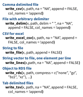
#readr::write_csv(df.chem_02, "df.chem_02.csv")
readr::write_csv(df.chem_02, paste0(dataFolder,"df.chem_02.csv"))
We can also use as_tibble() function of tibble package
df.chem_03<-tibble::as_tibble(read.csv(paste0(dataFolder,"PAHdata.csv"), check.names = FALSE))
str(df.chem_03)
tibble [20 × 23] (S3: tbl_df/tbl/data.frame)
$ Subject : chr [1:20] "P1" "P3" "P4" "P5" ...
$ Napthalene : num [1:20] 0.899 3.626 3.392 3.577 4.491 ...
$ 1-Methyl Napthalene : num [1:20] 4.97 4.69 3.54 4.75 5.11 ...
$ 2-Methyl Napthalene : num [1:20] 2.15 3.93 1.7 2.94 4 ...
$ Acenapthylene : num [1:20] 0.0131 3.0151 1.3859 3.3943 6.6593 ...
$ 1,2 Dimethyl napthalene : num [1:20] NA NA 1.24 2.64 2.14 ...
$ 1,6 Dimethyl Napthalene : num [1:20] 0.7 2.64 1.38 1.1 2.26 ...
$ Fluorene : num [1:20] 2.25 7.35 7.16 8.44 9.24 ...
$ 1,6,7 Trimethylnapthalene: num [1:20] 5.1 6.79 6.52 4.68 6.46 ...
$ Anthracene : num [1:20] 10.17 9.64 22.4 26.38 20.96 ...
$ Dibenzothiopene : num [1:20] 1.16 4.12 4.23 3.99 3.26 ...
$ 2-Methyl Anthracene : num [1:20] 0.541 4.519 8.401 13.01 4.49 ...
$ 1-Methylphenanthrene : num [1:20] 14.96 12.09 19.49 11.21 2.03 ...
$ 2-Methylphenanthrene : num [1:20] 5.48 18.25 36.43 16.46 10.8 ...
$ Pyrene : num [1:20] 4.85 14.94 10.11 26.06 20.87 ...
$ Fluoranthene : num [1:20] 4.48 9.72 9.8 19.05 20.09 ...
$ 1-Phenyl napthalene : num [1:20] 2.88 6.25 5.3 7.95 10.16 ...
$ 2-Phenyl napthalene : num [1:20] 3.41 8.74 3.7 12.85 15.1 ...
$ 1 Methylpyrene : num [1:20] 4.58 7.51 13.6 8.11 19.24 ...
$ Benzo(c)phenanthrene : num [1:20] 3.65 7.04 5.1 3.38 8.16 ...
$ Triphenylene/Chrysene : num [1:20] 1.74 5.14 3.16 5.71 6.75 ...
$ Benz(a)pyrene : num [1:20] NA 2.845 NA 5.07 0.587 ...
$ Benz(e)pyrene : num [1:20] NA 1.816 0.298 0.662 2.367 ...This tutorial provides an overview of the data import-export capabilities offered by the R package readr. By simplifying the process of reading and writing data in R, readr offers a seamless experience for handling various file formats. The tutorial begins by demonstrating how to use read_csv(), read_tsv(), and read_delim() functions to read data from CSV, TSV, and custom-delimited files respectively. The automatic data type inference and streamlined reading process make readr a valuable tool for handling diverse datasets. In addition, the tutorial covers the export functionalities of readr, demonstrating how to use write_csv(), write_tsv(), and write_delim() functions to write data frames to external files in a straightforward manner. The consistency in syntax across reading and writing functions simplifies the data import-export process. Another highlight is readr’s support for handling large datasets efficiently, making it an ideal choice for projects involving extensive data volumes. As you integrate readr into your data analysis workflow, it is recommended that you explore its additional features, such as custom column types, locale settings, and flexible options for handling missing or malformed data. Leveraging these capabilities will enhance your ability to handle various data scenarios. ## References