Simple Linear Regression is widely used in various fields for prediction, understanding relationships between variables, and making informed decisions based on observed data. In this tutorial, we will guide you through performing simple linear regression analysis step by step. We’ll cover everything you need to know, from understanding the underlying concepts to fitting regression models and interpreting the results using R, a versatile programming language for statistical analysis and data visualization. This tutorial is designed for beginners and assumes no prior knowledge of regression analysis or R programming. By the end of this tutorial, you will have a solid understanding of simple linear regression and be able to apply it to your own datasets. We will provide clear explanations, practical examples, and hands-on exercises to help you grasp the concepts effectively.
Introduction
Regression analysis is a powerful statistical tool that allows us to explore the complex relationships between variables. It helps us to understand how changes in one variable affect the other, quantify the strength of the relationship, and make predictions about future outcomes. By examining the data, we can identify patterns, trends, and anomalies that may not appear at first glance. This method is commonly used in economics, psychology, and finance to analyze large datasets and draw meaningful insights. With its ability to model complex relationships, regression analysis is an essential tool for any data scientist or researcher.
Linear regression is a statistical methodology that enables modeling the relationship between a dependent variable and one or more independent variables. The aim is to identify the linear relationship that best predicts the dependent variable based on the values of the independent variables.
Linear regression models are widely used in various fields, including economics, finance, biology, and social sciences, to analyze the relationship between variables and predict future outcomes. The technique is instrumental in identifying trends, patterns, and associations between variables, which can be used to develop hypotheses and test theories.
The ultimate objective of linear regression is to identify the linear equation that best describes the relationship between the independent and dependent variables. The equation can then be used to predict the dependent variable’s value based on the independent variables’ values. The model’s accuracy can be measured using various statistical measures, such as the coefficient of determination (R-squared) and the root mean squared error (RMSE). These measures indicate how well the model fits the data and how accurate the predictions are.
In conclusion, linear regression is a powerful statistical tool that can be used to gain insights into the relationship between variables, make predictions, and test hypotheses. Its wide range of applications and the accuracy of its predictions make it an indispensable tool in various fields.
Here are the key components of linear regression:
Dependent Variable (Y): This is the variable we want to predict or explain. It’s also known as the response variable.
Independent Variable(s) (X): These are the variables used to predict the dependent variable. If there’s only one independent variable, it’s a simple linear regression. If there are multiple, it’s a multiple linear regression.
Regression Equation: The linear regression equation is represented as \[ Y = b_0 +b_1X_1 + b_2X_2 + \ldots +b_n.X_n + \varepsilon\ \]where \(Y\) is the dependent variable, \(X_1, X_2,...X_n\) are the independent variables, \(b_0\) is the intercept, \(b_1, b_2,...b_n\) are coefficient and \(\varepsilon\) is the error term.
Coefficients: These are the weights assigned to each independent variable, representing the strength and direction of their impact on the dependent variable.
Residuals: Residuals are the differences between the actual and predicted values. The goal is to minimize these differences.
Assumptions: Linear regression assumes linearity, independence, homoscedasticity, and normality of residuals.
Ordinary Least Squares (OLS): This method is used to find the coefficients by minimizing the sum of squared residuals.
Linear regression analysis is based on six fundamental assumptions:
The dependent and independent variables show a linear relationship between the slope and the intercept.
The independent variable is not random.
The value of the residual (error) is zero.
The value of the residual (error) is constant across all observations.
The value of the residual (error) is not correlated across all observations.
The residual (error) values follow the normal distribution
Linear regression is widely used in various fields, such as economics, finance, biology, etc. It’s a simple yet powerful tool for predicting and understanding relationships between variables.
Simple Linear Regression
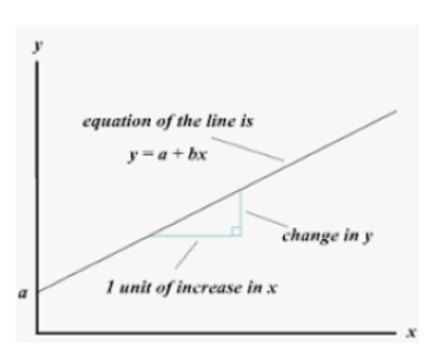
Simple Linear Regression is a statistical method used to model the relationship between a single dependent variable (usually denoted as \(Y\) and a single independent variable (usually denoted as \(X\)). The relationship is assumed to be linear and is represented by the equation of a straight line.
The general form of the simple linear regression model is given by:
\[ Y = b_0 +b_1X + \varepsilon\ \]
where \(Y\) is the dependent variable, \(X\) is the independent variable, \(b_0\) is the intercept, \(b_1\) is slope and \(\varepsilon\) is the error term.
The goal of simple linear regression is to estimate the values of \(b_0\) and \(b_1\) that minimize the sum of squared differences between the observed values of \(Y\) and the values predicted by the model.
The estimated coefficients, denoted as (\(\hat{b_0}\)) and (\(\hat{b_1}\)), are typically computed using the least squares method. Once the coefficients are estimated, the regression equation becomes:
\[ \hat{Y} = \hat{b_0}+\hat{b_1}X \]
This equation can be used to make predictions for the dependent variable \(Y\) based on new values of \(X\).
The goodness of fit of the model is often assessed using metrics such as the coefficient of determination (\(R^2\)), which indicates the proportion of the variance in the dependent variable that is explained by the independent variable. Here below formula for \(R^2\) is given by:
\[ R^2 = 1 - \frac{SS_{res}}{SS_{tot}} \]
where \(SS_{res}\) is the sum of squared residuals and \(SS_{tot}\) is the total sum of squares.
Simple Regression Analysis from Scratch
In this section, we will perform a simple linear regression analysis from scratch using R. We will create a dataset, calculate the coefficients for the regression line, make predictions, and evaluate the model’s performance.
Code
# Create a simple datasetx <-c(1, 2, 3, 4, 5)y <-c(2, 4, 5, 4, 5)# Calculate the means of x and ymean_x <-mean(x)mean_y <-mean(y)# Calculate the coefficients for the regression line: y = m * x + bnumerator <-sum((x - mean_x) * (y - mean_y))denominator <-sum((x - mean_x)^2)m <- numerator / denominatorb <- mean_y - m * mean_x# Display the coefficientscat("Slope (m):", m, "\n")
Slope (m): 0.6
Code
cat("Intercept (b):", b, "\n")
Intercept (b): 2.2
Code
# Make predictions using the regression liney_pred <- m * x + b# Calculate R-squared (R²)ss_total <-sum((y - mean_y)^2) # Total sum of squaresss_residual <-sum((y - y_pred)^2) # Residual sum of squaresr_squared <-1- (ss_residual / ss_total)# Display R² valuecat("R-squared (R²):", r_squared, "\n")
Simple linear regression analysis is a powerful statistical technique used to model the relationship between a dependent variable and one or more independent variables. In this tutorial, we will explore how to perform simple linear regression analysis using R, a popular programming language for statistical computing and data analysis. We will cover the following topics:
Check and Install Required R Packages
In these exercise we will use following R-Packages:
tydyverse: The tidyverse is a collection of R packages designed for data science.
broom:broom summarizes key information about models in tidy tibble()s. broom provides three verbs to make it convenient to interact with model objects:
report: report’s primary goal is to bridge the gap between R’s output and the formatted results contained in your manuscript.
stargazer:The Stargazer package is a great way to create tables to neatly represent your regression outputs nicely.
performance: The primary goal of the performance package is to fill this gap and to provide utilities for computing indices of model quality and goodness of fit.
jtools: This is a collection of tools for more efficiently understanding and sharing the results of (primarily) regression analyses. There are also a number of miscellaneous functions for statistical and programming purposes. Support for models produced by the survey and lme4 packages are points of emphasis.
relaimpo: Provides several metrics for assessing relative importance in linear models.
ggpmisc:Package ‘ggpmisc’ (Miscellaneous Extensions to ‘ggplot2’) is a set of extensions to R package ‘ggplot2’ (>= 3.0.0) with emphasis on annotations and plotting related to fitted models.
In this exercise we will fit a simple linear regression model to explore the relationship between soil organic carbon (SOC) and Normalized Vegetation Index (NDVI) using lm() function:
Code
slm.soc<-lm(SOC~NDVI, data=mf) # regression model
The summary() function is then used to display the summary of the linear model, including the estimated coefficients, standard errors, t-statistics, p-values, and \(R^2\) value.
Code
summary(slm.soc)
Call:
lm(formula = SOC ~ NDVI, data = mf)

Residuals:
   Min     1Q Median     3Q    Max
-9.543 -2.459 -0.722  1.362 18.614

Coefficients:
            Estimate Std. Error t value Pr(>|t|)
(Intercept)  -1.6432     0.5451  -3.014  0.00272 **
NDVI         18.2998     1.1703  15.637  < 2e-16 ***
---
Signif. codes:  0 '***' 0.001 '**' 0.01 '*' 0.05 '.' 0.1 ' ' 1

Residual standard error: 4.089 on 465 degrees of freedom
Multiple R-squared:  0.3446,    Adjusted R-squared:  0.3432
F-statistic: 244.5 on 1 and 465 DF,  p-value: < 2.2e-16
Create Regression Summary Table
With the tidy() function from the broom package, you can easily create standard regression output tables.
We can generate report for linear model using report() function of report package:
install.package(“report”)
Code
#library(report)report::report(slm.soc)
We fitted a linear model (estimated using OLS) to predict SOC with NDVI
(formula: SOC ~ NDVI). The model explains a statistically significant and
substantial proportion of variance (R2 = 0.34, F(1, 465) = 244.51, p < .001,
adj. R2 = 0.34). The model's intercept, corresponding to NDVI = 0, is at -1.64
(95% CI [-2.71, -0.57], t(465) = -3.01, p = 0.003). Within this model:

  - The effect of NDVI is statistically significant and positive (beta = 18.30,
95% CI [16.00, 20.60], t(465) = 15.64, p < .001; Std. beta = 0.59, 95% CI
[0.51, 0.66])

Standardized parameters were obtained by fitting the model on a standardized
version of the dataset. 95% Confidence Intervals (CIs) and p-values were
computed using a Wald t-distribution approximation.
Model Performance
The performance package provide utilities for computing indices of model quality and goodness of fit. These include measures like, model_performance %, root mean squared error (RMSE) or intraclass correlation coefficient (ICC) , but also functions to check (mixed) models for overdispersion, zero-inflation, convergence or singularity.
install.packages(“performance”)
Model performance summaries
model_performance computes indices of model performance for regression models. Depending on the model object, typical indices might be r-squared, AIC, BIC, RMSE, ICC or LOOIC.
AIC: AIC (Akaike Information Criterion) is a statistical measure used for model selection. It is a way to balance the goodness of fit of a model with the number of parameters in the model.
AICc: AICc (corrected Akaike Information Criterion) is a modification of the AIC statistic that is used to adjust for small sample sizes. AICc is calculated using the formula:
BIC: BIC (Bayesian Information Criterion) is another statistical measure used for model selection, similar to AIC. BIC is also based on the trade-off between model fit and model complexity, but it uses a different penalty for the number of parameters in the model.
RMSE: Root Mean Square Error (RMSE) is a commonly used metric to measure the accuracy of a predictive model. It is used to quantify the difference between the predicted values and the actual values in a dataset. RMSE is calculated by taking the square root of the mean of the squared differences between the predicted and actual values.
\(R^2\): \(R^2\), is a statistical measure that indicates how well a regression model fits the data. It is also known as the coefficient of determination.
Adjusted \(R^2\): Adjusted R2 is a modified version of the R2 statistic that adjusts for the number of independent variables in the regression model. It is used to evaluate the goodness of fit of a regression model, while accounting for the complexity of the model.
Sigma: The sigma of a regression model, also known as the residual standard error, is a measure of the variability of the errors in the regression model. It is a standard deviation of the residuals, which are the differences between the predicted values and the actual values.
R-squred and RMSE
R package performance has a generic r2() and performance_rmse() functions, which computes the \(R^2\) and RMSE for many different models,including linear, mixed effects and Bayesian regression models.
Code
# r2performance::r2(slm.soc)
# R2 for Linear Regression
       R2: 0.345
  adj. R2: 0.343
Code
# RMSEperformance::performance_rmse(slm.soc)
[1] 4.080156
Visualization of model assumptions
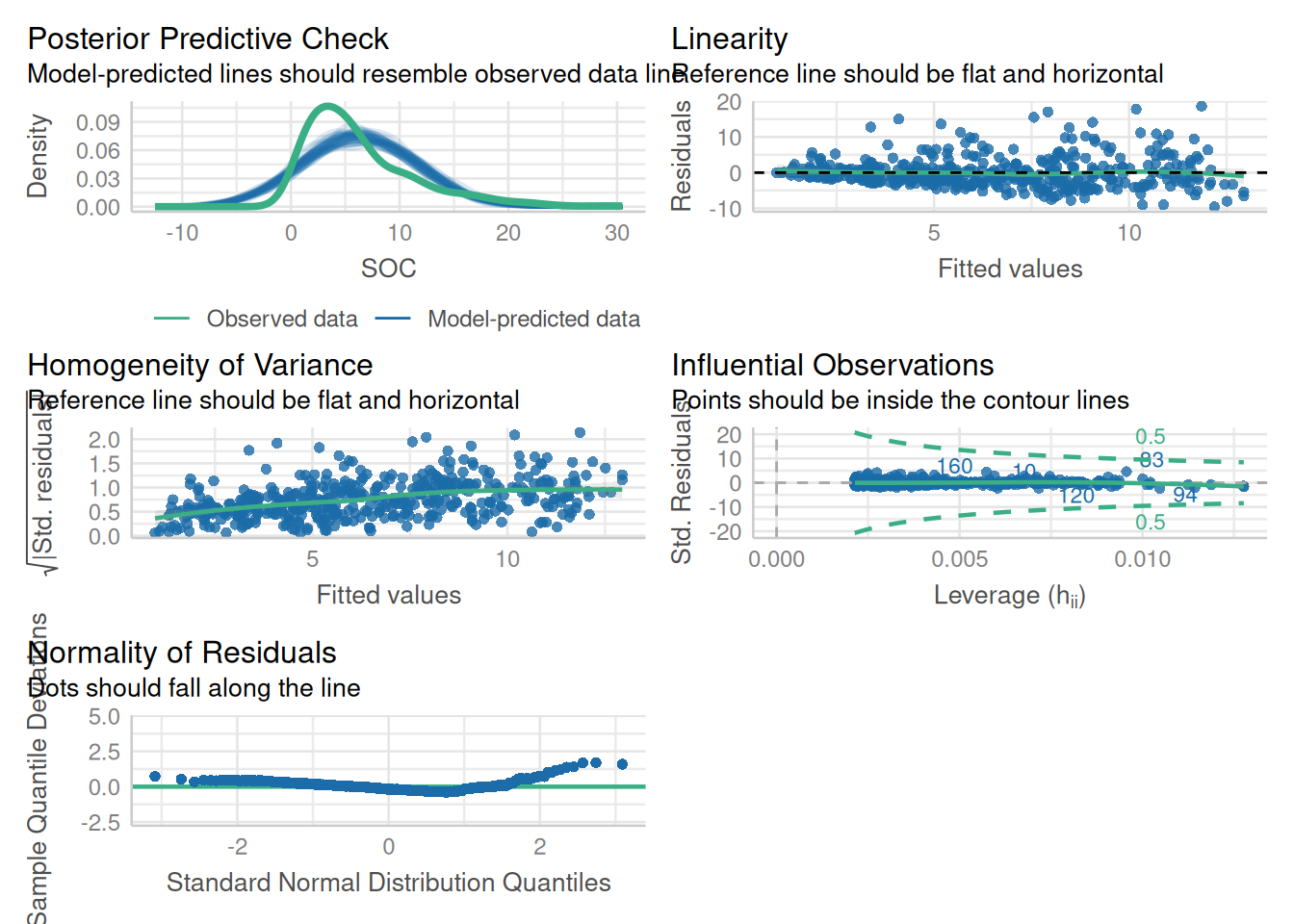
The package performance provides many functions to check model assumptions, like check_collinearity(), check_normality() or check_heteroscedasticity(). To get a comprehensive check, use check_model().
Posterior predictive: Posterior predictive checks for a linear model involve simulating data sets from the posterior distribution of the model parameters, and then comparing the simulated data sets to the observed data
Linearity: Linearity plots the residuals (i.e., the differences between the observed values and the predicted values) against the independent variable(s). If the plot shows a random pattern with no clear trend, then the linearity assumption is likely to hold. If the plot shows a pattern or trend, then the linearity assumption may be violated.
Homogeneity of variance: Homogeneity of variance can be assessed by examining a scatter plot of the residuals against the predicted values or against the independent variable(s). If the plot shows a random pattern with no clear trend, then the assumption of homogeneity of variance is likely to hold. If the plot shows a pattern or trend, such as increasing or decreasing variance, then the assumption of homogeneity of variance may be violated.
Influential observation : The influential observations in a linear regression model is an observation that has a strong effect on the estimated regression coefficients. These observations can have a large impact on the regression model and can affect the conclusions that are drawn from the analysis. Cook’s distance or the leverage statistic is generally use to measure statistical measures of influence. Observations that have high values of Cook’s distance or leverage may be influential.
Normality of residuals: It can be assessed by examining a histogram or a normal probability plot of the residuals. If the histogram shows a symmetric bell-shaped distribution, and the normal probability plot shows a roughly straight line, then the assumption of normality is likely to hold. If the histogram or normal probability plot shows departures from normality, such as skewness or outliers, then the assumption of normality may be violated.
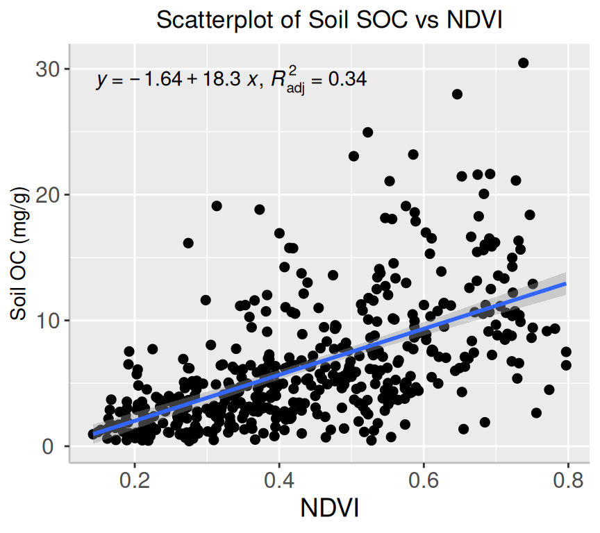
Visualize Linear Model
ggpmisc extends the capabilities of ggplot2 for visualization scatter plots of two variables. It provides additional functionality for annotation and customization of ggplot2 plots, including statistical annotations, highlighting subsets of data, and adding equations or text annotations.
stat_poly_eq() adds equation and R-squared values to a plot with a linear regression line.
install.package(ggmisc)
Code
#formula<-SOC~NDVIlibrary(ggpmisc)formula<-y~xggplot(mf, aes(x=NDVI, y=SOC)) +geom_point(size=2) +# draw fitted linegeom_smooth(method ="lm", formula = formula) +stat_poly_eq(use_label(c("eq", "adj.R2")), formula = formula) +# add plot titleggtitle("Scatterplot of Soil SOC vs NDVI") +theme(# center the plot titleplot.title =element_text(hjust =0.5),axis.line =element_line(colour ="gray"),# axis title font sizeaxis.title.x =element_text(size =14), # X and axis font sizeaxis.text.y=element_text(size=12,vjust =0.5, hjust=0.5),axis.text.x =element_text(size=12))+xlab("NDVI") +ylab("Soil OC (mg/g)")
Summary and Conclusion
This tutorial on simple linear regression analysis in R offers a comprehensive guide to help you understand and apply this statistical technique. By following this tutorial, you will gain a detailed understanding of the process involved in simple linear regression analysis. You will learn how to confidently handle data using R and perform regression analysis to identify relationships between variables. This tutorial will equip you with the knowledge and skills to make accurate predictions and draw valuable insights from your data.
Simple linear regression analysis is an essential tool in your data analysis toolkit. It enables you to investigate trends and patterns in your data and effectively inform decision-making processes. You will learn to interpret regression output, assess model fit and performance, and make predictions using your model. Additionally, you will understand how to test for assumptions, identify influential observations, and visualize them.
By the end of this tutorial, you will thoroughly understand how to use simple linear regression analysis in R. You will be well-equipped to explore relationships between variables, make predictions, and draw valuable insights from your data. Simple linear regression analysis is a versatile statistical technique that can be used across various industries, making it an indispensable tool for data analysts and researchers alike.