Code
packages <- c(
          'tidyverse',
          'data.table'
) ![]()

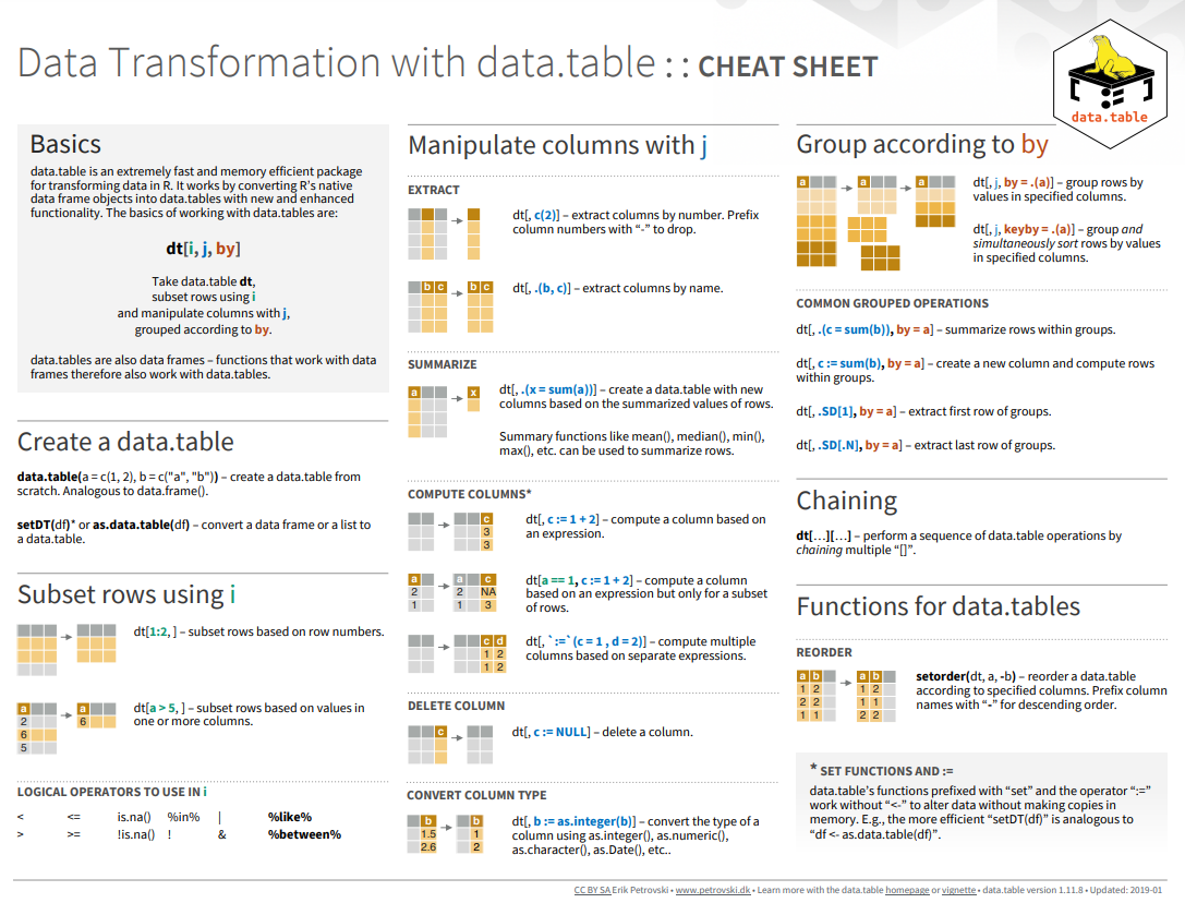
The data.table is a powerful and widely used package in the R programming language. It provides an alternative to the default data.frame for handling tabular data. One of the primary reasons for its popularity is its exceptional performance, especially when dealing with large datasets. The package’s concise syntax is another benefit of using data.table. It allows for complex data manipulations and transformations with less code, making it a favorite among Data Scientists.

{Data.table} is one of the most downloaded packages in R. It’s well-liked by developers and analysts, who consider it one of the best things that has happened to the R programming language in terms of speed. The package’s syntax differs somewhat from the regular R data.frame. However, it is quite intuitive once you get the hang of it. This makes it easy to use and understand, and once you learn it, you may never want to revert to using the base R data.frame syntax. In summary, data.table is a powerful, fast, and intuitive package for managing tabular data in R. Its popularity among Data Scientists is a testament to its usefulness and efficiency. With data.table, you can write less code and achieve faster results, making it a go-to package for working with large datasets.
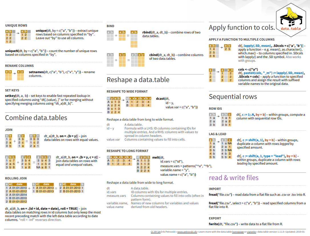
Here below data transformation with data.table:
packages <- c(
'tidyverse',
'data.table'
) #| warning: false
#| error: false
# Install missing packages
new_packages <- packages[!(packages %in% installed.packages()[,"Package"])]
if(length(new_packages)) install.packages(new_packages)# Verify installation
cat("Installed packages:\n")Installed packages:print(sapply(packages, requireNamespace, quietly = TRUE)) tidyverse data.table
TRUE TRUE # Load packages with suppressed messages
invisible(lapply(packages, function(pkg) {
suppressPackageStartupMessages(library(pkg, character.only = TRUE))
}))# Check loaded packages
cat("Successfully loaded packages:\n")Successfully loaded packages:print(search()[grepl("package:", search())]) [1] "package:data.table" "package:lubridate" "package:forcats"
[4] "package:stringr" "package:dplyr" "package:purrr"
[7] "package:readr" "package:tidyr" "package:tibble"
[10] "package:ggplot2" "package:tidyverse" "package:stats"
[13] "package:graphics" "package:grDevices" "package:utils"
[16] "package:datasets" "package:methods" "package:base" In this exercise we will use following CSV files:
usa_division.csv: USA division names with IDs
usa_state.csv: USA State names with ID and division ID.
usa_corn_production.csv: USA grain crop production by state from 2012-2022
All data set use in this exercise can be downloaded from my Dropbox or from my Github accounts.
We will use fread() function of data.table package to import data as a tidy data. When it comes to working with data.tables, it’s important to realize that the process is different from working with data.frames. Before diving in and using this package, it’s essential to understand the differences between the two. One of the most useful functions of data.table is fread(), which is a faster and more efficient version of read.csv(). It’s worth noting that fread() can work with local files on your computer, as well as files hosted on the internet. In fact, it’s been shown to be at least 20 times faster than read.csv(), which can be a huge advantage when dealing with large datasets. This dataset is stored as a csv file and can be easily imported using fread(). By using this function, you’ll be able to import the data quickly and efficiently into your R environment.
div.dt<-fread("https://github.com/zia207/r-colab/raw/main/Data/R_Beginners/usa_division.csv")
state.dt<-fread("https://github.com/zia207/r-colab/raw/main/Data/R_Beginners/usa_state.csv")class(div.dt)[1] "data.table" "data.frame"When data is imported, it can be stored in various formats. In this case, the data is stored as a data.table. It is worth noting that a data.table is a type of data structure that inherits from the data.frame class. This means that the data.table itself can be considered a data.frame. By default, data.tables have some unique features that make them efficient when working with large datasets. For example, they have optimized memory usage and fast operations for querying and processing data.
corn.df<-read_csv("https://github.com/zia207/r-colab/raw/main/Data/R_Beginners/usa_corn_production.csv")Rows: 465 Columns: 3
── Column specification ────────────────────────────────────────────────────────
Delimiter: ","
dbl (3): STATE_ID, YEAR, MT
ℹ Use `spec()` to retrieve the full column specification for this data.
ℹ Specify the column types or set `show_col_types = FALSE` to quiet this message.class(corn.df)[1] "spec_tbl_df" "tbl_df" "tbl" "data.frame" You can use as.data.table() or setDT() to convert data.frame to data.table:
corn.dt<-as.data.table(corn.df)
# Alternately, use setDT() to convert it to data.table in place.
corn.dt<-setDT(corn.df)
class(corn.dt)
[1] "data.table" "data.frame"Conversely, use as.data.frame(dt) or setDF(dt)to convert a data.table to a data.frame
Important: The data.table() does not have any rownames. So if the data.frame has any rownames, you need to store it as a separate column before converting to data.table.
The data.table package offers a faster and more efficient implementation of the merge() function. It is designed to handle large datasets with ease, making it ideal for big data management and analysis. With data.table, you can merge two or more datasets based on common columns and perform operations like filtering, sorting, and aggregating on the merged data. The syntax of data.table’s merge() function is quite similar to base R’s merge(), making it easy to learn and use for anyone familiar with the latter. Data analysts and data scientists can use data.table to speed up their data manipulation tasks and save time on their projects.
We will join state, division and USA corn production data one by one e using merge() function with all=T argument:
corn_state = merge(state.dt, corn.dt, by='STATE_ID', all = T) |>
             glimpse()
Rows: 465
Columns: 5
$ STATE_ID <int> 1, 1, 1, 1, 1, 1, 1, 1, 1, 1, 1, 4, 4, 4, 4, 4, 4, 4, 4, 4…
$ STATE_NAME <chr> "Alabama", "Alabama", "Alabama", "Alabama", "Alabama", "Al…
$ DIVISION_ID <int> 2, 2, 2, 2, 2, 2, 2, 2, 2, 2, 2, 4, 4, 4, 4, 4, 4, 4, 4, 4…
$ YEAR <dbl> 2012, 2013, 2014, 2015, 2016, 2017, 2018, 2019, 2020, 2021…
$ MT <dbl> 734352.8, 1101529.2, 1151061.8, 914829.3, 960170.7, 996875…corn_state_div = merge(corn_state, div.dt, by='DIVISION_ID', all = T) |>
glimpse()Rows: 465
Columns: 6
$ DIVISION_ID <int> 1, 1, 1, 1, 1, 1, 1, 1, 1, 1, 1, 1, 1, 1, 1, 1, 1, 1, 1,…
$ STATE_ID <int> 17, 17, 17, 17, 17, 17, 17, 17, 17, 17, 17, 18, 18, 18, …
$ STATE_NAME <chr> "Illinois", "Illinois", "Illinois", "Illinois", "Illinoi…
$ YEAR <dbl> 2012, 2013, 2014, 2015, 2016, 2017, 2018, 2019, 2020, 20…
$ MT <dbl> 32672475, 53352977, 59693152, 51120199, 57296535, 559070…
$ DIVISION_NAME <chr> "East North Central", "East North Central", "East North …We can run multiple merge() functions in a series with pipe %>% or | > operator:
corn.usa = merge(state.dt, corn.dt, by='STATE_ID', all = T)  |>
          merge(div.dt, by='DIVISION_ID', all = T)  |>
          glimpse()
Rows: 465
Columns: 6
$ DIVISION_ID <int> 1, 1, 1, 1, 1, 1, 1, 1, 1, 1, 1, 1, 1, 1, 1, 1, 1, 1, 1,…
$ STATE_ID <int> 17, 17, 17, 17, 17, 17, 17, 17, 17, 17, 17, 18, 18, 18, …
$ STATE_NAME <chr> "Illinois", "Illinois", "Illinois", "Illinois", "Illinoi…
$ YEAR <dbl> 2012, 2013, 2014, 2015, 2016, 2017, 2018, 2019, 2020, 20…
$ MT <dbl> 32672475, 53352977, 59693152, 51120199, 57296535, 559070…
$ DIVISION_NAME <chr> "East North Central", "East North Central", "East North …We merge multiple data.table with a custom merge() and Reduce() functions to repeatedly merge multiple data.tables stored in a list.
# read four files
fips<-fread("https://github.com/zia207/r-colab/raw/main/Data/R_Beginners/LBC_Data_ID.csv")
rate<-fread("https://github.com/zia207/r-colab/raw/main/Data/R_Beginners/LBC_Data_Rate.csv")
smoking<-fread("https://github.com/zia207/r-colab/raw/main/Data/R_Beginners/LBC_Data_Smoking.csv")
pm25<-fread("https://github.com/zia207/r-colab/raw/main/Data/R_Beginners/LBC_Data_PM25.csv")# create a list
dt_list <- list(fips, rate, smoking, pm25)
# merge function
merge_func <- function(...) merge(..., all = TRUE, by='FIPS')
# use Reduce() merge all dt together
LBC.usa <- Reduce(merge_func, dt_list) |>
glimpse()Rows: 3,152
Columns: 9
$ FIPS <int> 1001, 1003, 1005, 1007, 1009, 1011, 1013, 1013, 1013, 1013, …
$ REGION_ID <int> 3, 3, 3, 3, 3, 3, 3, 3, 3, 3, 3, 3, 3, 3, 3, 3, 3, 3, 3, 3, …
$ STATE <chr> "Alabama", "Alabama", "Alabama", "Alabama", "Alabama", "Alab…
$ County <chr> "Autauga County", "Baldwin County", "Barbour County", "Bibb …
$ X <dbl> 872679.2, 789777.5, 997211.0, 822862.5, 863725.2, 964066.8, …
$ Y <dbl> 1094433.0, 884557.1, 1033023.8, 1141553.6, 1255735.2, 105519…
$ LBC_Rate <dbl> 54.2, 48.1, 48.9, 54.2, 55.2, 66.6, 38.3, 38.3, 38.3, 38.3, …
$ Smoking <dbl> 22.4, 20.8, 24.7, 26.1, 24.1, 25.3, 26.0, 26.0, 26.0, 26.0, …
$ PM25 <dbl> 9.20, 7.89, 8.58, 9.28, 9.08, 8.79, 8.46, 8.46, 8.46, 8.46, …In data.table, all set() functions change their input by reference. That is, no copy is made at all, other than temporary working memory which is as large as one column. The only other data.table operator that modifies input by reference is :=.
Now we will organize DIVISION_FIPS, DIVISION_NAME, STATE_FIPS, STATE_NAME, DIVISION_NAME, YEAR, MT with setcolorder() function.
corn.usa<-setcolorder(corn.usa,
                        c("DIVISION_ID",
                       "DIVISION_NAME",
                        "STATE_ID",
                        "STATE_NAME",
                        "YEAR",
                        "MT"))
head(corn.usa)
Key: <DIVISION_ID>
DIVISION_ID DIVISION_NAME STATE_ID STATE_NAME YEAR MT
<int> <char> <int> <char> <num> <num>
1: 1 East North Central 17 Illinois 2012 32672475
2: 1 East North Central 17 Illinois 2013 53352977
3: 1 East North Central 17 Illinois 2014 59693152
4: 1 East North Central 17 Illinois 2015 51120199
5: 1 East North Central 17 Illinois 2016 57296535
6: 1 East North Central 17 Illinois 2017 55907082setnames() operates on data.table and data.frame not other types like list and vector. It can be used to change names by name with built-in checks and warnings
We will rename STAT_ID to SATE_FIPS.
setnames(corn.usa, "STATE_ID", "STATE_FIPS")
names(corn.usa)
[1] "DIVISION_ID" "DIVISION_NAME" "STATE_FIPS" "STATE_NAME"
[5] "YEAR" "MT" In data.table, the j argument within square brackets ([ ]) is used to select columns. This argument allows you to specify the columns that you want to select from your dataset. You can select columns by either their names or indices. If you want to select columns by their names, you can simply specify the column names within the square brackets, separated by commas.
Following code select STATE_NAME column, but return it as a vector.
corn.state <- corn.usa[,STATE_NAME]
head(corn.state)
[1] "Illinois" "Illinois" "Illinois" "Illinois" "Illinois" "Illinois"Following code select STATE_NAME column, but return but return as a data.table instead.
corn.state <- corn.usa[,list(STATE_NAME)]
head(corn.state)
STATE_NAME
<char>
1: Illinois
2: Illinois
3: Illinois
4: Illinois
5: Illinois
6: Illinoisdata.table also allows wrapping columns with .() instead of list(). It is an alias to list(); they both mean the same.
corn.state <- corn.usa[,list(STATE_NAME, YEAR, MT)]
## alternatively
corn.state <- corn.usa[,.(STATE_NAME, YEAR, MT)]
head(corn.state)
STATE_NAME YEAR MT
<char> <num> <num>
1: Illinois 2012 32672475
2: Illinois 2013 53352977
3: Illinois 2014 59693152
4: Illinois 2015 51120199
5: Illinois 2016 57296535
6: Illinois 2017 55907082Filtering a data.table in R is a powerful and flexible operation that allows you to extract subsets of data based on specific conditions. The i argument within square brackets is used to specify these conditions. The conditions can involve one or more columns in the data.table and can be combined using logical operators such as &, |, and !. For example, you can filter a data.table to extract only the rows where a particular column meets a certain criterion, or where two or more columns satisfy a complex condition. Additionally, you can use the .SD variable to refer to the subset of data.table that matches the filtering criteria. This enables you to perform further operations on the filtered data, such as summarization or aggregation.
df.01<-corn.usa[DIVISION_NAME == "East North Central",]
levels(as.factor(df.01$STATE_NAME))
[1] "Illinois" "Indiana" "Michigan" "Ohio" "Wisconsin"Filtering by multiple criteria within a single logical expression - select data from East North Central, South Central and Middle Atlantic Division
df.02<- corn.usa[DIVISION_NAME %in%c("East North Central",
                                     "East South Central",
                                     "Middle Atlantic"),]
levels(as.factor(df.02$STATE_NAME))
[1] "Alabama" "Illinois" "Indiana" "Kentucky" "Michigan"
[6] "Mississippi" "New Jersey" "New York" "Ohio" "Pennsylvania"
[11] "Tennessee" "Wisconsin" or we can use | which represents OR in the logical condition, any of the two conditions.
df.03<- corn.usa [DIVISION_NAME == "East North Central" | DIVISION_NAME == "Middle Atlantic",]
levels(as.factor(df.03$STATE_NAME))
[1] "Illinois" "Indiana" "Michigan" "New Jersey" "New York"
[6] "Ohio" "Pennsylvania" "Wisconsin" Following filter create a files for the Middle Atlantic Division only with New York state.
df.ny<-corn.usa[DIVISION_NAME == "Middle Atlantic" & STATE_NAME == "New York",]
head(df.ny)
Key: <DIVISION_ID>
DIVISION_ID DIVISION_NAME STATE_FIPS STATE_NAME YEAR MT
<int> <char> <int> <char> <num> <num>
1: 3 Middle Atlantic 36 New York 2012 2314570
2: 3 Middle Atlantic 36 New York 2013 2401189
3: 3 Middle Atlantic 36 New York 2014 2556391
4: 3 Middle Atlantic 36 New York 2015 2143111
5: 3 Middle Atlantic 36 New York 2016 1867761
6: 3 Middle Atlantic 36 New York 2017 1983464Following filters will select State where corn production (MT) is greater than the global average of production
mean.prod <- corn.usa[MT > mean(MT, na.rm = TRUE),]
levels(as.factor(mean.prod$STATE_NAME))
[1] "Illinois" "Indiana" "Iowa" "Kansas" "Michigan"
[6] "Minnesota" "Missouri" "Nebraska" "North Dakota" "Ohio"
[11] "South Dakota" "Wisconsin" We use will & in the following filters to select states or rows where MT is greater than the global average of for the year 2017
mean.prod.2017 <- corn.usa[MT > mean(MT, na.rm = TRUE) & YEAR ==2017,]
levels(as.factor(mean.prod.2017$STATE_NAME))
[1] "Illinois" "Indiana" "Iowa" "Kansas" "Minnesota"
[6] "Missouri" "Nebraska" "North Dakota" "Ohio" "South Dakota"
[11] "Wisconsin" Following command will select counties starting with “A”. filter() with grepl() is used to search for pattern matching.
state.a <- corn.usa[grepl("^A", STATE_NAME),]
levels(as.factor(state.a $STATE_NAME))
[1] "Alabama" "Arizona" "Arkansas"Data.table is a powerful package in R that offers an efficient and fast way to perform operations on large datasets. One of its main features is the ability to summarize data using various functions such as sum(), mean(), count(), and many others. To use these functions, you simply need to enclose them within square brackets ([ ]). This will allow you to summarize the data based on certain criteria or conditions, and quickly retrieve important information such as the total sum, average, or count of a specific column or group of columns. By utilizing data.table, you can easily analyze your data in a more efficient and streamlined manner.
# mean
LBC.usa[,mean(LBC_Rate)]
[1] 47.17349# Median
LBC.usa[,median(LBC_Rate)][1] 46.35For multiple variables:
In data.table, you can calculate the mean of multiple columns by specifying them within the j argument and using the lapply() function to apply the mean() function across those columns. Here’s an example:
LBC.usa[, lapply(.SD, mean), .SDcols = c("LBC_Rate", "Smoking", "PM25")] LBC_Rate Smoking PM25
<num> <num> <num>
1: 47.17349 21.47538 7.132129Here, .SD refers to the Subset of Data and .SDcols specifies the columns on which the operation needs to be performed (in this case, columns “LBC_Rate”, “Smoking”, “PM25”). The lapply() function applies the mean() function across these selected columns to calculate their mean
You can compute both the mean and standard deviation of multiple columns simultaneously within a data.table in R.
summary_stats <- LBC.usa[, lapply(.SD,
                           function(x) c(mean = mean(x), sd = sd(x))),
                           .SDcols = c("LBC_Rate", "Smoking", "PM25")]
summary_stats
LBC_Rate Smoking PM25
<num> <num> <num>
1: 47.17349 21.475381 7.132129
2: 13.46195 3.292703 1.761107In data.table, you can use the by argument to group your data based on one or more columns, and then calculate summary statistics for each group. This is useful when you want to perform calculations on subsets of your data. For example, you can group your data by a categorical variable, such as ‘gender’ or ‘age group’, and then calculate the mean, standard deviation, count, or other summary statistics for each group. The resulting data table will have one row for each group, with the summary statistics calculated for that group. This allows you to quickly compare different groups and identify any patterns or trends in your data.
We can calculate mean and SD of LBC rate by regions:
# Calculate mean grouped by 'Region_ID'
mean.lbc<-LBC.usa[, lapply(.SD, mean), .SDcols = c("LBC_Rate", "Smoking", "PM25"), by = REGION_ID]
# Calculate mean grouped by 'Region_ID'
sd.lbc<-LBC.usa[, lapply(.SD, sd), .SDcols = c("LBC_Rate", "Smoking", "PM25"), by = REGION_ID]
mean.lbc
REGION_ID LBC_Rate Smoking PM25
<int> <num> <num> <num>
1: 3 52.23064 22.74744 7.766694
2: 4 33.48258 18.62512 4.364589
3: 1 42.96590 19.65945 7.215853
4: 2 46.37865 21.19829 7.318738We can also calculate statistics of multiple variables using following code:
LBC.usa[, lapply(.SD,
                     function(x) c(mean = mean(x), sd = sd(x))),
                      .SDcols = c("LBC_Rate", "Smoking", "PM25"),   by = REGION_ID]
REGION_ID LBC_Rate Smoking PM25
<int> <num> <num> <num>
1: 3 52.230641 22.747444 7.766694
2: 3 13.780368 3.199699 1.031159
3: 4 33.482585 18.625121 4.364589
4: 4 9.901008 3.063832 1.147293
5: 1 42.965899 19.659447 7.215853
6: 1 7.758635 2.244585 1.435032
7: 2 46.378653 21.198292 7.318738
8: 2 10.654334 2.696246 1.803687We can calculate summary statistics by group using following code:
LBC.usa[, as.list(summary(LBC_Rate)), by = REGION_ID] REGION_ID Min. 1st Qu. Median Mean 3rd Qu. Max.
<int> <num> <num> <num> <num> <num> <num>
1: 3 13.96 43.1500 51.300 52.23064 59.65 134.7
2: 4 10.10 26.4850 33.235 33.48258 39.80 67.1
3: 1 25.20 37.7000 43.700 42.96590 48.00 69.7
4: 2 18.90 38.2925 45.400 46.37865 52.90 93.8One of the key features of data.table is the ability to create a new column by assigning values to it within the square brackets. This can be done using the := operator, which allows you to assign a value to a column by reference.
In this exercise we will create a new column (MT_1000) in df.corn dataframe dividing MT column by 1000
corn.usa[, MT_1000 := MT / 10000] |>
    glimpse()
Rows: 465
Columns: 7
$ DIVISION_ID <int> 1, 1, 1, 1, 1, 1, 1, 1, 1, 1, 1, 1, 1, 1, 1, 1, 1, 1, 1,…
$ DIVISION_NAME <chr> "East North Central", "East North Central", "East North …
$ STATE_FIPS <int> 17, 17, 17, 17, 17, 17, 17, 17, 17, 17, 17, 18, 18, 18, …
$ STATE_NAME <chr> "Illinois", "Illinois", "Illinois", "Illinois", "Illinoi…
$ YEAR <dbl> 2012, 2013, 2014, 2015, 2016, 2017, 2018, 2019, 2020, 20…
$ MT <dbl> 32672475, 53352977, 59693152, 51120199, 57296535, 559070…
$ MT_1000 <dbl> 3267.2475, 5335.2977, 5969.3152, 5112.0199, 5729.6535, 5…In R, there are several packages that provide functions for pivoting data frames. The reshape2 package offers melt() and cast() functions that make it easy to reshape data. The tidyr package provides gather() and spread() functions that are useful for reshaping data from wide to long or vice versa.
Finally, the data.table package provides the dcast() and melt() function that can be used to pivot data frames in a more efficient way, especially for large data sets. To perform pivoting, you need to specify the variables that will be used as rows, columns, and values. The rows variable will be the key variable that you use to group the data. The columns variable will be used to generate new columns in the output, and the values variable will be used to populate the cells in the output. Overall, pivoting a data frame is an essential skill for data analysts and scientists, and R provides powerful tools to make this transformation easy and efficient.
First we will drop data of several states:
 # Drop state where reporting years less than 11
state_list <- c("Connecticut",
                "Maine",
                "Massachusetts",
                "Nevada",
                "New Hampshire",
                "Rhode Island",
                "Vermont")

slected_state<-corn.usa[!STATE_NAME %in% state_list]
head(slected_state)
Key: <DIVISION_ID>
DIVISION_ID DIVISION_NAME STATE_FIPS STATE_NAME YEAR MT MT_1000
<int> <char> <int> <char> <num> <num> <num>
1: 1 East North Central 17 Illinois 2012 32672475 3267.248
2: 1 East North Central 17 Illinois 2013 53352977 5335.298
3: 1 East North Central 17 Illinois 2014 59693152 5969.315
4: 1 East North Central 17 Illinois 2015 51120199 5112.020
5: 1 East North Central 17 Illinois 2016 57296535 5729.654
6: 1 East North Central 17 Illinois 2017 55907082 5590.708The dcast() function is a highly efficient data reshaping tool provided by the data.table package. It is used for converting long-form data into wide-form data, and it can handle very large data sets with ease.
One of the main advantages of using dcast() is its speed and memory efficiency due to its optimized algorithms, the function is capable of handling large data sets in RAM without slowing down or causing memory issues. This makes it an excellent choice for data analysts and scientists who work with large-scale data.
Another advantage of dcast() is its ability to handle multiple value.var columns. This means that users can easily cast multiple columns of their dataset simultaneously, without having to perform multiple reshaping operations. Furthermore, the function supports multiple functions to fun.aggregate, which allows users to compute multiple summary statistics on their data at once.
Overall, dcast() is a powerful and efficient tool that can greatly simplify the data reshaping process for users working with large and complex data sets.
#
slected_state  |>  dcast(YEAR ~ STATE_NAME,
             value.var = "MT") |>
glimpse()
Rows: 11
Columns: 42
$ YEAR <dbl> 2012, 2013, 2014, 2015, 2016, 2017, 2018, 2019, 2020,…
$ Alabama <dbl> 734352.8, 1101529.2, 1151061.8, 914829.3, 960170.7, 9…
$ Arizona <dbl> 158504.4, 229297.9, 149359.9, 192034.1, 273064.4, 158…
$ Arkansas <dbl> 3142400, 4110445, 2517527, 2045951, 3236004, 2765825,…
$ California <dbl> 823003.5, 873298.1, 398166.0, 239280.6, 469924.8, 339…
$ Colorado <dbl> 3412162, 3261024, 3745682, 3426641, 4071581, 4722109,…
$ Delaware <dbl> 610394.2, 733692.3, 853485.1, 799837.4, 708189.4, 820…
$ Florida <dbl> 116846.2, 263513.5, 137167.2, 179079.5, 147327.8, 151…
$ Georgia <dbl> 1417395, 2067034, 1338651, 1237934, 1425015, 1095306,…
$ Idaho <dbl> 668690.3, 528728.9, 406421.5, 368065.4, 477545.2, 592…
$ Illinois <dbl> 32672475, 53352977, 59693152, 51120199, 57296535, 559…
$ Indiana <dbl> 15163839, 26211898, 27554359, 20879902, 24037543, 237…
$ Iowa <dbl> 47675777, 54363950, 60135135, 63645600, 69612376, 661…
$ Kansas <dbl> 9531853, 12802276, 14382239, 14736842, 17746393, 1743…
$ Kentucky <dbl> 2642756, 6175066, 5739179, 5723430, 5654339, 5516155,…
$ Louisiana <dbl> 2329049, 2944270, 1812894, 1694015, 2305172, 2290185,…
$ Maryland <dbl> 1348049, 1685633, 1911451, 1583012, 1544402, 1834993,…
$ Michigan <dbl> 7980085, 8779974, 9038051, 8518086, 8135542, 7633357,…
$ Minnesota <dbl> 34912873, 32875940, 29917700, 36293436, 39219671, 375…
$ Mississippi <dbl> 3332021, 3710628, 2279135, 2178165, 3035968, 2400427,…
$ Missouri <dbl> 6286832, 11054664, 15969315, 11109531, 14491465, 1403…
$ Montana <dbl> 158504.4, 219086.6, 190510.1, 139707.4, 139707.4, 115…
$ Nebraska <dbl> 32823613, 40996495, 40694219, 42998120, 43179740, 427…
$ `New Jersey` <dbl> 257772.8, 282462.9, 315052.8, 268847.8, 261506.8, 296…
$ `New Mexico` <dbl> 185683.8, 183397.7, 237756.6, 182889.7, 156218.3, 146…
$ `New York` <dbl> 2314570, 2401189, 2556391, 2143111, 1867761, 1983464,…
$ `North Carolina` <dbl> 2437005, 3102012, 2615322, 2095357, 3080167, 3029872,…
$ `North Dakota` <dbl> 10722414, 10058931, 7968909, 8323512, 13123857, 11404…
$ Ohio <dbl> 11125787, 16530177, 15557814, 12669681, 13328084, 141…
$ Oklahoma <dbl> 824273.5, 1141790.3, 1082859.2, 917496.4, 1075746.8, …
$ Oregon <dbl> 270778.3, 171916.3, 188223.9, 143263.6, 227850.0, 236…
$ Pennsylvania <dbl> 3327576, 4042369, 4029161, 3509957, 3112934, 3762447,…
$ `South Carolina` <dbl> 960678.7, 1097719.0, 832147.9, 614204.4, 1129089.6, 1…
$ `South Dakota` <dbl> 13597338, 20392705, 20000000, 20315231, 20979730, 187…
$ Tennessee <dbl> 2072749, 3209714, 3584637, 2966877, 3183550, 3083977,…
$ Texas <dbl> 5078998, 6736436, 7481203, 6755487, 8226224, 7965861,…
$ Utah <dbl> 144228.8, 133865.1, 113798.0, 74705.3, 128911.8, 8941…
$ Virginia <dbl> 915718.4, 1408250.4, 1289118.1, 1226884.8, 1278195.5,…
$ Washington <dbl> 628048.2, 573435.3, 600741.7, 409596.6, 507391.8, 457…
$ `West Virginia` <dbl> 113798.0, 134423.9, 136252.8, 131579.0, 128911.8, 127…
$ Wisconsin <dbl> 10058931, 11160079, 12323715, 12497460, 14559033, 129…
$ Wyoming <dbl> 216419.4, 216140.0, 210323.1, 238290.0, 257645.8, 248…dcast() function supports multiple functions to fun.aggregate, which allows users to compute multiple summary statistics on their data at once.
dt.wider<-dcast(slected_state,
                YEAR ~ DIVISION_NAME,
                fun.aggregate = mean,
                value.var = 'MT')
head(dt.wider)
Key: <YEAR>
YEAR East North Central East South Central Middle Atlantic Mountain
<num> <num> <num> <num> <num>
1: 2012 15400224 2195470 1966640 706313.3
2: 2013 23207021 3549234 2242007 681648.6
3: 2014 24833418 3188503 2300202 721978.7
4: 2015 21137066 2945825 1973972 660333.3
5: 2016 23471347 3208507 1747401 786382.0
6: 2017 22885745 2999359 2014284 867571.9
Pacific South Atlantic West North Central West South Central
<num> <num> <num> <num>
1: 573943.3 989985.5 22221529 2843680
2: 539549.9 1311534.8 26077851 3733235
3: 395710.5 1139199.4 27009645 3223621
4: 264046.9 983486.0 28203182 2853237
5: 401722.2 1180162.2 31193319 3710787
6: 344509.9 1173961.1 29733322 3499511In R’s data.table, it’s possible to transform wide data into long format using the melt() function. This function is useful for reshaping data when it’s needed to transform a dataset into a format that is more suitable for analysis or visualization. To use the melt() function, you first need to specify the data.table object that contains the data you want to reshape. Then, you need to set the variables that you want to retain as the id.vars argument, which will keep these variables in the reshaped dataset. Finally, you will need to specify the variables that you want to reshape as the measure.vars argument, which will be used to create the new variables in the reshaped dataset.
The melt() function can be used to pivot a data frame from a wide format to a long format.
dt.longer<-dt.wider |>
               melt(id.vars = "YEAR",
               value.name = "MT",
               variable.name = "DIVISION_NAME",)
head(dt.longer)
YEAR DIVISION_NAME MT
<num> <fctr> <num>
1: 2012 East North Central 15400224
2: 2013 East North Central 23207021
3: 2014 East North Central 24833418
4: 2015 East North Central 21137066
5: 2016 East North Central 23471347
6: 2017 East North Central 22885745This tutorial explores data wrangling using the R package “data.table,” a powerful framework for managing large datasets. We will cover data filtering, column selection, grouping, and summarization. Advanced features include indexing, fast joins, and efficient data manipulation. With data. table, you can handle large datasets and complex operations. Practice with diverse datasets to streamline your workflows using the power of data.table.