Data Wrangling with {dplyr} and {tidyr}

In the upcoming section, you will delve deeper into data manipulation using two of the most widely used and versatile R-packages: {tidyr} and {dplyr}. Both these packages are part of the {tidyverse}, a comprehensive suite of R packages specially designed for data science applications. By mastering the functionalists of these two packages, you will be able to seamlessly transform, clean, and manipulate data in a streamlined and efficient manner. The {tidyr} package provides a set of tools to tidy data in a consistent and structured manner. In contrast, the {dplyr} package offers a range of functions to filter, sort, group, and summarize data frames efficiently. With the combined power of these two packages, you will be well-equipped to handle complex data manipulation tasks and derive meaningful insights from your data.

{tidyr} - Package

{tidyr} is a powerful data manipulation package that enables users to create `tidy** data, a specific format that makes it easy to work with, model, and visualize data. Tidy data follows a set of principles for organizing data into tables, where each column represents a variable, and each row represents an observation. The variables should have clear, descriptive names that are easy to understand, and the observations should be organized in a logical order. Tidy data is essential because it makes it easier to perform data analysis and visualization. Data in this format can be easily filtered, sorted, and summarized, which is particularly important when working with large datasets. Moreover, it allows users to apply a wide range of data analysis techniques, including regression, clustering, and machine learning, without having to worry about data formatting issues. Tidy data is the preferred format for many data analysis tools and techniques, including the popular R programming language.

{tidyr} package provides a suite of functions for cleaning, reshaping, and transforming data into a tidy format. It allows users to split, combine, and pivot data frames, which are essential operations when working with messy data. Overall, tidyr is a powerful tool that helps users to create tidy data, which is a structured and organized format that makes it easier to analyze and visualize data. Tidy data is a fundamental concept in data science and is widely used in many data analysis tools and techniques.

tidyr() functions fall into five main categories:

Pivotting which converts between long(pivot_longer()) and wide forms (pivot_wider()), replacing
Rectangling, which turns deeply nested lists (as from JSON) into tidy tibbles.
Nesting converts grouped data to a form where each group becomes a single row containing a nested data frame
Splitting and combining character columns. Use separate() and extract() to pull a single character column into multiple columns;
Make implicit missing values explicit with complete(); make explicit missing values implicit with drop_na(); replace missing values with next/previous value with fill(), or a known value with replace_na().

{dplyr} - Package

dplyr provides data manipulation grammar and a set of functions to efficiently clean, process, and aggregate data. It offers a tibble data structure, which is similar to a data frame but designed for easier use and better efficiency. Also, it provides a set of verbs for data manipulation, such as filter(), arrange(), select(), mutate(), and summarize(), to perform various data operations. Additionally, dplyr has a chainable syntax with pipe (%>% or |>), making it easy to execute multiple operations in a single line of code. Finally, it also supports working with remote data sources, including databases and big data systems.

On the other hand, tidyr helps to create tidy data that is easy to manipulate, model, and visualize. This type of data follows a set of rules for organizing variables, values, and observations into tables, where each column represents a variable, and each row represents an observation. Tidy data makes it easier to perform data analysis and visualization and is the preferred format for many data analysis tools and techniques.

In addition to data frames/tibbles, dplyr makes working with following packages:

dtplyr: for large, in-memory datasets. Translates your dplyr code to high performance data.table code.

dbplyr: for data stored in a relational database. Translates your dplyr code to SQL.

sparklyr: for very large datasets stored in Apache Spark.

In addition to tidyr, and dplyr, there are five packages (including stringr and forcats) which are designed to work with specific types of data:

lubridate for dates and date-times.
hms for time-of-day values.
blob for storing blob (binary) data

Cheat-sheet

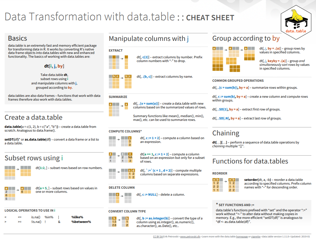
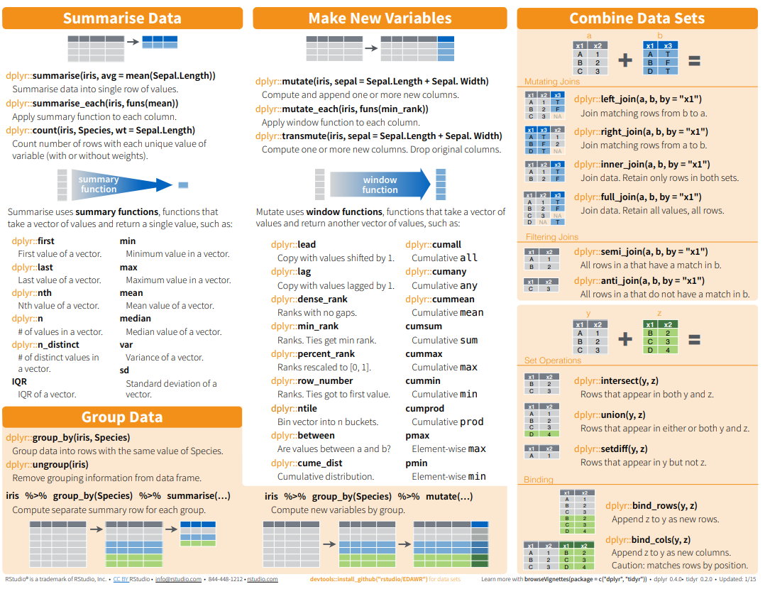
Here below data Wrangling with dplyr and tidyr Cheat Sheets:

{fig-dplyr_tidyr_02}

Check and Install Required R Packages

Code

packages <- c(
          'tidyverse'
)

#| warning: false
#| error: false

# Install missing packages
new_packages <- packages[!(packages %in% installed.packages()[,"Package"])]
if(length(new_packages)) install.packages(new_packages)

Verify Installtion

Code

# Verify installation
cat("Installed packages:\n")

Installed packages:

Code

print(sapply(packages, requireNamespace, quietly = TRUE))

tidyverse 
     TRUE

Load Packages

Code

# Load packages with suppressed messages
invisible(lapply(packages, function(pkg) {
  suppressPackageStartupMessages(library(pkg, character.only = TRUE))
}))

Check Loaded Packages

Code

# Check loaded packages
cat("Successfully loaded packages:\n")

Successfully loaded packages:

Code

print(search()[grepl("package:", search())])

 [1] "package:lubridate" "package:forcats"   "package:stringr"  
 [4] "package:dplyr"     "package:purrr"     "package:readr"    
 [7] "package:tidyr"     "package:tibble"    "package:ggplot2"  
[10] "package:tidyverse" "package:stats"     "package:graphics" 
[13] "package:grDevices" "package:utils"     "package:datasets" 
[16] "package:methods"   "package:base"

Data

In this exercise we will use following CSV files:

usa_division.csv: USA division names with IDs
usa_state.csv: USA State names with ID and division ID.
usa_corn_production.csv: USA grain crop production by state from 2012-2022
gp_soil_data.csv: Soil carbon with co-variate from four states in the Greatplain region in the USA
usa_geochemical_raw.csv: Soil geochemical data for the USA, but not cleaned

All data set use in this exercise can be downloaded from here

We will use read_csv() function of readr package to import data as a tidy data.

Code

div<-read_csv("https://raw.githubusercontent.com/zia207/Data/main/CSV_files/usa_division.csv")
state<-read_csv("https://raw.githubusercontent.com/zia207/Data/main/CSV_files/usa_state.csv")
corn<-read_csv("https://raw.githubusercontent.com/zia207/Data/main/CSV_files/usa_corn_production.csv")
soil<-read_csv("https://raw.githubusercontent.com/zia207/Data/main/CSV_files/gp_soil_data.csv")
head(soil)

# A tibble: 6 × 19
     ID  FIPS STATE_ID STATE  COUNTY Longitude Latitude   SOC   DEM Aspect Slope
  <dbl> <dbl>    <dbl> <chr>  <chr>      <dbl>    <dbl> <dbl> <dbl>  <dbl> <dbl>
1     1 56041       56 Wyomi… Uinta…     -111.     41.1  15.8 2229.   159.  5.67
2     2 56023       56 Wyomi… Linco…     -111.     42.9  15.9 1889.   157.  8.91
3     3 56039       56 Wyomi… Teton…     -111.     44.5  18.1 2423.   169.  4.77
4     4 56039       56 Wyomi… Teton…     -111.     44.4  10.7 2484.   198.  7.12
5     5 56029       56 Wyomi… Park …     -111.     44.8  10.5 2396.   201.  7.95
6     6 56039       56 Wyomi… Teton…     -111.     44.1  17.0 2361.   209.  9.66
# ℹ 8 more variables: TPI <dbl>, KFactor <dbl>, MAP <dbl>, MAT <dbl>,
#   NDVI <dbl>, SiltClay <dbl>, NLCD <chr>, FRG <chr>

Pipe Operator

At the beginning of this tutorial, I would like to provide you with a comprehensive overview of the Pipe Operator. This operator is a crucial tool for data wrangling in R. It is denoted by the symbols %>% or | > (keyboard shortcut shift+ctrl M) and requires the use of R 4.1 or higher. The Pipe Operator has been an integral part of the magrittr package for R for some time now. It allows us to take the output of one function and use it as an argument in another function, which helps us chain together a sequence of analysis steps.

To put it simply, suppose we have two functions, A and B. The output of function A can be passed directly to function B using the Pipe Operator. This way, we can avoid the need to store the intermediate results in variables, which can make our code more concise and easier to read.

In this tutorial, we will provide an example of how to use the Pipe Operator in a real-world scenario. We will demonstrate how it can help us to perform a sequence of data manipulation steps efficiently. So, stay tuned to learn more about this essential operator, and how you can use it to improve your data analysis skills in R.

Some Important Functions

Join

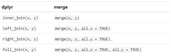
In R programming language, there are several functions to merge two dataframes. The base::merge() function is one such function that can be used to merge dataframes. This function is available in the join() function of the dplyr package. The base::merge() function can merge two dataframes based on one or more common columns.

Before merging two dataframes, it’s important to ensure that the dataframes have a common column (or columns) to merge on. These columns are called “key” variables. The most important condition for joining two dataframes is that the column type of “key” variables should be the same in both dataframes. If the column types are different, the merge operation might result in unexpected errors.

In R, there are different types of base::merge() functions available for different types of merges such as left, right, inner, and outer. Additionally, the dplyr package provides several join() functions like inner_join(), left_join(), right_join(), and full_join(). These functions can be used to merge dataframes based on different conditions. For example, inner_join() returns only the rows that have matching values in both dataframes, left_join() returns all rows from the left dataframe and the matching rows from the right dataframe, and so on.

Types of base::merge() and several join() function of dplyr available in R are:

inner_join() is a function in the dplyr library that performs an inner join on two data frames. An inner join returns only the rows that have matching values in both data frames. If there is no match in one of the data frames for a row in the other data frame, the result will not contain that row.

inner_join(x, y, …..)

We will join state, division and USA corn production data one by one e using inner_join() function:

Code

corn_state = dplyr::inner_join(corn, state)

Code

corn_state_div = dplyr::inner_join(corn_state, div)

We can run multiple inner_join() functions in a series with pipe %>%or |> operator:

Code

mf.usa = dplyr::inner_join(corn, state)  |>  
         dplyr::inner_join(div)  |> 
         glimpse()

Rows: 465
Columns: 6
$ STATE_ID      <dbl> 1, 1, 1, 1, 1, 1, 1, 1, 1, 1, 1, 4, 4, 4, 4, 4, 4, 4, 4,…
$ YEAR          <dbl> 2012, 2013, 2014, 2015, 2016, 2017, 2018, 2019, 2020, 20…
$ MT            <dbl> 734352.8, 1101529.2, 1151061.8, 914829.3, 960170.7, 9968…
$ STATE_NAME    <chr> "Alabama", "Alabama", "Alabama", "Alabama", "Alabama", "…
$ DIVISION_ID   <dbl> 2, 2, 2, 2, 2, 2, 2, 2, 2, 2, 2, 4, 4, 4, 4, 4, 4, 4, 4,…
$ DIVISION_NAME <chr> "East South Central", "East South Central", "East South …

Tip

glimpse() function is similar to the print() function, but with one significant difference. In glimpse(), columns are displayed vertically, and data is displayed horizontally. This makes it easier to view all the columns in a data frame. It is similar to the str() function, but it shows more data. Additionally, it always displays the underlying data, even when used with a remote data source.

Relocate

The relocate() function can be used to rearrange the positions of columns in a tabular dataset. This function works in a similar way to the select() function, making it easy to move blocks of columns at once. By using the relocate() function, you can specify the new positions of columns in the dataset and ensure that they are in the desired order. This can be particularly useful when working with large datasets that require reorganization of columns to suit specific needs.

Now we will organize DIVISION_FIPS, DIVISION_NAME, STATE_FIPS, STATE_NAME, DIVISION_NAME, YEAR, MT with relocate() function:

relocate(.data, …, .before = NULL, .after = NULL)

Code

mf.usa<-dplyr::relocate(mf.usa, 
                        DIVISION_ID, 
                        DIVISION_NAME, 
                        STATE_ID,   
                        STATE_NAME, 
                        YEAR, 
                        MT,  
                        .after =  DIVISION_ID)
head(mf.usa)

# A tibble: 6 × 6
  DIVISION_ID DIVISION_NAME      STATE_ID STATE_NAME  YEAR       MT
        <dbl> <chr>                 <dbl> <chr>      <dbl>    <dbl>
1           2 East South Central        1 Alabama     2012  734353.
2           2 East South Central        1 Alabama     2013 1101529.
3           2 East South Central        1 Alabama     2014 1151062.
4           2 East South Central        1 Alabama     2015  914829.
5           2 East South Central        1 Alabama     2016  960171.
6           2 East South Central        1 Alabama     2017  996876.

Explore regions names with levels() function:

Code

levels(as.factor(mf.usa$DIVISION_NAME))

[1] "East North Central" "East South Central" "Middle Atlantic"   
[4] "Mountain"           "New England"        "Pacific"           
[7] "South Atlantic"     "West North Central" "West South Central"

Rename

The rename() function can be used to change the name of an individual variable. The syntax for this is new_name = old_name. On the other hand, the rename_with() function can be used to rename columns in a dataframe. This function accepts a function that is used to generate new names for the columns. The function should take a string as input and return a string as output. The rename_with() function is a powerful tool that allows you to rename columns based on specific criteria or patterns. With this function, you can easily rename columns in a dataframe without having to manually change each column name.

We will rename STAT_ID to SATE_FIPS.

Code

df.usa <- mf.usa  |>  
        dplyr::rename("STATE_FIPS" = "STATE_ID")    
names(df.usa)

[1] "DIVISION_ID"   "DIVISION_NAME" "STATE_FIPS"    "STATE_NAME"   
[5] "YEAR"          "MT"

Join, Relocate and Rename functions with Pipe

We can run inner_join(), relocate(), and rename() in a single line with pipe:

Code

df.corn = dplyr::inner_join(corn, state) |>
          dplyr::inner_join(div)  |>
          dplyr::relocate(DIVISION_ID,
                          DIVISION_NAME, 
                          STATE_ID,   
                          STATE_NAME, 
                          YEAR, 
                          MT,
                         .after =  DIVISION_ID) |>
          dplyr::rename("STATE_FIPS" = "STATE_ID")  |>
        glimpse()

Rows: 465
Columns: 6
$ DIVISION_ID   <dbl> 2, 2, 2, 2, 2, 2, 2, 2, 2, 2, 2, 4, 4, 4, 4, 4, 4, 4, 4,…
$ DIVISION_NAME <chr> "East South Central", "East South Central", "East South …
$ STATE_FIPS    <dbl> 1, 1, 1, 1, 1, 1, 1, 1, 1, 1, 1, 4, 4, 4, 4, 4, 4, 4, 4,…
$ STATE_NAME    <chr> "Alabama", "Alabama", "Alabama", "Alabama", "Alabama", "…
$ YEAR          <dbl> 2012, 2013, 2014, 2015, 2016, 2017, 2018, 2019, 2020, 20…
$ MT            <dbl> 734352.8, 1101529.2, 1151061.8, 914829.3, 960170.7, 9968…

Select

The dplyr::select() function is a powerful and versatile tool used to extract a subset of columns from a data frame in R programming. This function enables you to select specific columns based on their name or position within the data frame. By using the dplyr package, you can perform common data manipulation tasks efficiently and effectively. This package provides a set of functions that are designed to work seamlessly with one another to streamline the data manipulation process.

Overview of selection features

Tidyverse selections implement a dialect of R where operators make it easy to select variables:

:for selecting a range of consecutive variables.
!for taking the complement of a set of variables.
&and |for selecting the intersection or the union of two sets of variables.
c() for combining selections.

In addition, you can use **selection helpers**. Some helpers select specific columns:

everything(): Matches all variables.
last_col(): Select last variable, possibly with an offset.
group_cols(): Select all grouping columns.

Other helpers select variables by matching patterns in their names:

starts_with(): Starts with a prefix.
ends_with(): Ends with a suffix.
contains(): Contains a literal string.
matches(): Matches a regular expression.
num_range(): Matches a numerical range like x01, x02, x03.

Or from variables stored in a character vector:

all_of(): Matches variable names in a character vector. All names must be present, otherwise an out-of-bounds error is thrown.
any_of(): Same as all_of(), except that o error is thrown for names that don’t

Or using a predicate function:

where(): Applies a function to all variables and selects those for which the function returns TRUE.

Ww will use select() to create a dataframe with state names, year and production:

Code

df.state <- df.corn |> 
           dplyr::select(STATE_NAME, 
                         YEAR,  
                         MT,) |> 
           glimpse()

Rows: 465
Columns: 3
$ STATE_NAME <chr> "Alabama", "Alabama", "Alabama", "Alabama", "Alabama", "Ala…
$ YEAR       <dbl> 2012, 2013, 2014, 2015, 2016, 2017, 2018, 2019, 2020, 2021,…
$ MT         <dbl> 734352.8, 1101529.2, 1151061.8, 914829.3, 960170.7, 996875.…

Filter

The filter() function in R is a powerful tool for working with data frames. It allows you to subset a data frame by retaining only the rows that meet specific conditions.

When using filter(), you must provide one or more conditions that each row must satisfy. For example, you may want to filter a data frame to only include rows where a certain column meets a certain condition, such as all rows where the value of a column is greater than 10.

To specify conditions, you can use logical operators such as ==, !=, <, >, <=, and >=. You can also use the %in% operator to check if a value is contained in a list.

It’s important to note that when using filter(), each row must satisfy all the given conditions to be retained. If a condition evaluates to FALSE or NA, that row will be dropped from the resulting data frame.

Unlike base subsetting with [, if a condition evaluates to NA, the row will also be dropped. This is because R treats NA as an undefined value, and so it can’t determine whether the condition is satisfied or not.

Overall, filter() is a useful function for working with data frames in R, and its ability to subset data based on specific conditions can be very helpful when working with large data sets.

Code

df.01<-df.corn |> 
       dplyr::filter(DIVISION_NAME == "East North Central")
levels(as.factor(df.01$STATE_NAME))

[1] "Illinois"  "Indiana"   "Michigan"  "Ohio"      "Wisconsin"

Filtering by multiple criteria within a single logical expression - select data from East North Central, South Central and Middle Atlantic Division

Code

df.02<- df.corn  |>  
        dplyr::filter(DIVISION_NAME %in%c("East North Central",
                                          "East South Central", 
                                          "Middle Atlantic")) 
levels(as.factor(df.02$STATE_NAME))

 [1] "Alabama"      "Illinois"     "Indiana"      "Kentucky"     "Michigan"    
 [6] "Mississippi"  "New Jersey"   "New York"     "Ohio"         "Pennsylvania"
[11] "Tennessee"    "Wisconsin"

or we can use | which represents OR in the logical condition, any of the two conditions.

Code

df.03<- df.usa |> 
        dplyr::filter(DIVISION_NAME == "East North Central" | DIVISION_NAME == "Middle Atlantic")
levels(as.factor(df.03$STATE_NAME))

[1] "Illinois"     "Indiana"      "Michigan"     "New Jersey"   "New York"    
[6] "Ohio"         "Pennsylvania" "Wisconsin"

Following filter create a files for the Middle Atlantic Division only with New York state.

Code

df.ny<-df.corn  |>  
         dplyr::filter(DIVISION_NAME == "Middle Atlantic" & STATE_NAME == "New York")
head(df.ny)

# A tibble: 6 × 6
  DIVISION_ID DIVISION_NAME   STATE_FIPS STATE_NAME  YEAR       MT
        <dbl> <chr>                <dbl> <chr>      <dbl>    <dbl>
1           3 Middle Atlantic         36 New York    2012 2314570.
2           3 Middle Atlantic         36 New York    2013 2401189.
3           3 Middle Atlantic         36 New York    2014 2556391 
4           3 Middle Atlantic         36 New York    2015 2143111.
5           3 Middle Atlantic         36 New York    2016 1867761.
6           3 Middle Atlantic         36 New York    2017 1983464.

Following filters will select State where corn production (MT) is greater than the global average of production

Code

mean.prod <- df.corn |> 
              dplyr::filter(MT > mean(MT, na.rm = TRUE))
levels(as.factor(mean.prod$STATE_NAME))

 [1] "Illinois"     "Indiana"      "Iowa"         "Kansas"       "Michigan"    
 [6] "Minnesota"    "Missouri"     "Nebraska"     "North Dakota" "Ohio"        
[11] "South Dakota" "Wisconsin"

We use will & in the following filters to select states or rows where MT is greater than the global average of for the year 2017

Code

mean.prod.2017 <- df.corn |> 
              dplyr::filter(MT > mean(MT, na.rm = TRUE) & YEAR ==2017)
levels(as.factor(mean.prod.2017$STATE_NAME))

 [1] "Illinois"     "Indiana"      "Iowa"         "Kansas"       "Minnesota"   
 [6] "Missouri"     "Nebraska"     "North Dakota" "Ohio"         "South Dakota"
[11] "Wisconsin"

Following command will select counties starting with “A”. filter() with grepl() is used to search for pattern matching.

Code

state.a <- df.corn  |>  
          dplyr::filter(grepl("^A", STATE_NAME))
levels(as.factor(state.a $STATE_NAME))

[1] "Alabama"  "Arizona"  "Arkansas"

Summarize

In the dplyr package, there is a very useful function called summarize(). Its purpose is to condense multiple values in a data frame into a single summary value. Essentially, it takes a data frame as input and returns a smaller data frame that contains various summary statistics. For instance, you can use summarize to calculate the mean, sum, count, or any other statistical measure you need to analyze your data. This function is often used in conjunction with other dplyr functions, such as filter and mutate, to manipulate and analyze data effectively. Overall, summarize is a powerful tool that can help you streamline your data analysis tasks and quickly extract valuable insights from your data.

Center: mean(), median()
Spread: sd(), IQR(), mad()
Range: min(), max(), quantile()
Position: first(), last(), nth(),
Count: n(), n_distinct()
Logical: any(), all()

summarise() and summarize() are synonyms.

Code

# mean
summarize(df.corn, Mean=mean(MT))

# A tibble: 1 × 1
      Mean
     <dbl>
1 8360402.

Code

# median
summarise(df.corn, Median=median(MT))

# A tibble: 1 × 1
    Median
     <dbl>
1 2072749.

The scoped variants (_if, _at, _all) of summarise() make it easy to apply the same transformation to multiple variables. There are three variants.

summarise_at() affects variables selected with a character vector or vars()
summarise_all() affects every variable
summarise_if() affects variables selected with a predicate function

Following summarise_at()function mean of SOC from USA soil data (soil).

Code

soil  |> 
    dplyr::summarise_at("SOC", mean, na.rm = TRUE)

# A tibble: 1 × 1
    SOC
  <dbl>
1  6.35

For multiple variables:

Code

soil  |> 
    dplyr::summarise_at(c("SOC", "NDVI"), mean, na.rm = TRUE)

# A tibble: 1 × 2
    SOC  NDVI
  <dbl> <dbl>
1  6.35 0.437

The summarise_if() variants apply a predicate function (a function that returns TRUE or FALSE) to determine the relevant subset of columns.

Here we apply mean() to the numeric columns:

Code

soil  |> 
    dplyr::summarise_if(is.numeric, mean, na.rm = TRUE)

# A tibble: 1 × 15
     ID   FIPS STATE_ID Longitude Latitude   SOC   DEM Aspect Slope     TPI
  <dbl>  <dbl>    <dbl>     <dbl>    <dbl> <dbl> <dbl>  <dbl> <dbl>   <dbl>
1  238. 29151.     29.1     -104.     38.9  6.35 1632.   165.  4.84 0.00937
# ℹ 5 more variables: KFactor <dbl>, MAP <dbl>, MAT <dbl>, NDVI <dbl>,
#   SiltClay <dbl>

Code

soil  |> 
   dplyr::summarise(across(where(is.numeric), ~ mean(.x, na.rm = TRUE)))

# A tibble: 1 × 15
     ID   FIPS STATE_ID Longitude Latitude   SOC   DEM Aspect Slope     TPI
  <dbl>  <dbl>    <dbl>     <dbl>    <dbl> <dbl> <dbl>  <dbl> <dbl>   <dbl>
1  238. 29151.     29.1     -104.     38.9  6.35 1632.   165.  4.84 0.00937
# ℹ 5 more variables: KFactor <dbl>, MAP <dbl>, MAT <dbl>, NDVI <dbl>,
#   SiltClay <dbl>

It is better to select first our target numerical columns and then apply summarise_all():

Code

soil  |> 
    # First select  numerical columns
    dplyr::select(SOC, DEM, NDVI, MAP, MAT) |> 
    # get mean of all these variables
    dplyr::summarise_all(mean, na.rm = TRUE)

# A tibble: 1 × 5
    SOC   DEM  NDVI   MAP   MAT
  <dbl> <dbl> <dbl> <dbl> <dbl>
1  6.35 1632. 0.437  501.  8.88

Mutate

The mutate() function is a powerful tool that can be used to create new columns in a data frame by using expressions that manipulate the values of existing columns or variables. It is a part of the dplyr package in R and is used extensively in data manipulation tasks.

When you use the mutate() function, you can specify new column names and the expressions that will be used to generate the column values. The expressions can use the values from one or more existing columns or variables, and can include arithmetic operations, logical operators, and other functions.

The mutate() function returns a new data frame with the added columns and the same number of rows as the original dataframe. This means that the original data frame is not modified, and the new data frame can be used for further analysis or visualization tasks.

Overall, the mutate() function is a versatile tool that can simplify complex data manipulation tasks and streamline your data analysis workflow.

In this exercise we will create a new column (MT_1000) in df.corn dataframe dividing MT column by 1000

Code

df.corn  |> 
    # get mean of all these variables
    dplyr::mutate(MT_1000 = MT / 10000)  |> 
    glimpse()

Rows: 465
Columns: 7
$ DIVISION_ID   <dbl> 2, 2, 2, 2, 2, 2, 2, 2, 2, 2, 2, 4, 4, 4, 4, 4, 4, 4, 4,…
$ DIVISION_NAME <chr> "East South Central", "East South Central", "East South …
$ STATE_FIPS    <dbl> 1, 1, 1, 1, 1, 1, 1, 1, 1, 1, 1, 4, 4, 4, 4, 4, 4, 4, 4,…
$ STATE_NAME    <chr> "Alabama", "Alabama", "Alabama", "Alabama", "Alabama", "…
$ YEAR          <dbl> 2012, 2013, 2014, 2015, 2016, 2017, 2018, 2019, 2020, 20…
$ MT            <dbl> 734352.8, 1101529.2, 1151061.8, 914829.3, 960170.7, 9968…
$ MT_1000       <dbl> 73.43528, 110.15292, 115.10618, 91.48293, 96.01707, 99.6…

Group by

The function group_by() is used to group a data frame by one or more variables. Once the data is grouped, you can perform various operations on it, such as aggregating with summarize(), transforming with mutate(), or filtering with filter(). The output of grouping is a grouped tibble, which is a data structure that retains the grouping structure and allows you to perform further operations on the grouped data.

We can calculate global mean of USA corn production by division:

Code

df.corn |>   
          dplyr::group_by(DIVISION_NAME) |> 
          dplyr::summarize(Prod_MT = mean(MT))

# A tibble: 9 × 2
  DIVISION_NAME        Prod_MT
  <chr>                  <dbl>
1 East North Central 22246702.
2 East South Central  3143670.
3 Middle Atlantic     2036263.
4 Mountain             712629.
5 New England           15203.
6 Pacific              384083.
7 South Atlantic      1163065.
8 West North Central 27893388.
9 West South Central  3163740.

We can also apply the group_by(), summarize() and mutate() functions with pipe to calculate mean of corn production in 1000 MT by division for the year 2022

Code

df.corn |> 
          dplyr::filter(YEAR==2020) |> 
          dplyr::group_by(DIVISION_NAME) |> 
          dplyr::summarize(Prod_MT = mean(MT)) |> 
          dplyr::mutate(Prod_1000_MT = Prod_MT / 1000)

# A tibble: 8 × 3
  DIVISION_NAME        Prod_MT Prod_1000_MT
  <chr>                  <dbl>        <dbl>
1 East North Central 22746952.       22747.
2 East South Central  3350119.        3350.
3 Middle Atlantic     1929554.        1930.
4 Mountain             651221.         651.
5 Pacific              391731.         392.
6 South Atlantic      1223075.        1223.
7 West North Central 28281091.       28281.
8 West South Central  3009964.        3010.

We can also apply the group_by() and summarize() functions to calculate statistic of multiple variable:

Code

soil |> 
  group_by(STATE) |> 
  summarize(SOC = mean(SOC),
            NDVI = mean(NDVI),
            MAP = mean(MAP),
            MAT = mean(MAT))

# A tibble: 4 × 5
  STATE        SOC  NDVI   MAP   MAT
  <chr>      <dbl> <dbl> <dbl> <dbl>
1 Colorado    7.29 0.482  473.  6.93
2 Kansas      7.43 0.570  742. 12.6 
3 New Mexico  3.51 0.301  388. 11.6 
4 Wyoming     6.90 0.390  419.  5.27

Following code will identify the states where corn production data has not reported for the all years.

Code

df.corn |>  
  dplyr::group_by(STATE_NAME) |> 
  dplyr::summarise(n = n()) |> 
  dplyr::filter(n < 11)

# A tibble: 7 × 2
  STATE_NAME        n
  <chr>         <int>
1 Connecticut       2
2 Maine             2
3 Massachusetts     2
4 Nevada            2
5 New Hampshire     2
6 Rhode Island      2
7 Vermont           2

Pivoting Data-frame

Pivoting a DataFrame is a data manipulation technique that involves reorganizing the structure of the data to create a new view. This technique is particularly useful when working with large datasets because it can help to make the data more manageable and easier to analyze. In R, pivoting a DataFrame typically involves using the dplyr or tidyr packages to transform the data from a long format to a wide format or vice versa. This allows for easier analysis of the data and can help to highlight patterns, trends, and relationships that might otherwise be difficult to see. Overall, pivoting a DataFrame is an important tool in the data analyst’s toolkit and can be used to gain valuable insights into complex datasets.

In R, there are multiple ways to pivot a data frame, but the most common methods are:

tidyr::pivot_wider: The pivot_wider() function is used to reshape a data frame from a long format to a wide format, in which each row becomes a variable, and each column is an observation.

tidyr::pivot_longer: This is a relatively new function in the tidyr library that makes it easy to pivot a data frame from wide to long format. It is used to reshape a data frame from a wide format to a long format, in which each column becomes a variable, and each row is an observation.

tidyr::spread(): This function is also used to pivot data from long to wide format. It creates new columns from the values of one column, based on the values of another column.

tidy::gather() : This function is used to pivot data from wide to long format. It collects values of multiple columns into a single column, based on the values of another column.

pivot_wider

pivot_wider() convert a dataset wider by increasing the number of columns and decreasing the number of rows.

Code

corn.wider = df.corn  |> 
           dplyr::select (STATE_FIPS,STATE_NAME, YEAR, MT) |> 
           # Drop state where reporting years less than 11 
           dplyr::filter(STATE_NAME!= 'Connecticut', 
                        STATE_NAME!= 'Maine',                        
                        STATE_NAME!= 'Massachusetts', 
                        STATE_NAME!= 'Nevada',
                        STATE_NAME!= 'New Hampshire', 
                        STATE_NAME!= 'Rhode Island', 
                        STATE_NAME!= 'Vermont') %>%
           tidyr::pivot_wider(names_from = YEAR, values_from = MT)

pivot_longer

The pivot_longer() function can be used to pivot a data frame from a wide format to a long format.

Code

corn.longer<- corn.wider |> 
               tidyr::pivot_longer(cols= c("2012", "2013", "2014", "2015", "2016", "2017",                                              "2018", "2019", "2020", "2021",  "2022"),
                          names_to = "YEAR", # column need to be wider
                          values_to = "MT") # data
head(corn.longer)

# A tibble: 6 × 4
  STATE_FIPS STATE_NAME YEAR        MT
       <dbl> <chr>      <chr>    <dbl>
1          1 Alabama    2012   734353.
2          1 Alabama    2013  1101529.
3          1 Alabama    2014  1151062.
4          1 Alabama    2015   914829.
5          1 Alabama    2016   960171.
6          1 Alabama    2017   996876.

Following command combined select(), rename(), summarize() and pivot_longer() the data:

Code

soil |> 
  # First select  numerical columns
  dplyr::select(SOC, DEM, NDVI, MAP, MAT) |> 
  # get summary statistics
  dplyr::summarise_all(funs(min = min, 
                      q25 = quantile(., 0.25), 
                      median = median, 
                      q75 = quantile(., 0.75), 
                      max = max,
                      mean = mean, 
                      sd = sd)) |>  
  # create a nice looking table
   tidyr::pivot_longer(everything(), names_sep = "_", names_to = c( "variable", ".value"))

# A tibble: 5 × 8
  variable     min      q25   median      q75      max     mean      sd
  <chr>      <dbl>    <dbl>    <dbl>    <dbl>    <dbl>    <dbl>   <dbl>
1 SOC        0.408    2.77     4.97     8.71    30.5      6.35    5.05 
2 DEM      259.    1175.    1593.    2238.    3618.    1632.    770.   
3 NDVI       0.142    0.308    0.417    0.557    0.797    0.437   0.162
4 MAP      194.     354.     434.     591.    1128.     501.    207.   
5 MAT       -0.591    5.87     9.17    12.4     16.9      8.88    4.10

Spread

tidyr::gather() is equivalent to tidyr::pivot_longer()

Code

df.corn |> 
  dplyr::select (STATE_FIPS, YEAR, STATE_NAME, MT)  |> 
  tidyr::spread(YEAR, MT)

# A tibble: 48 × 13
   STATE_FIPS STATE_NAME   `2012`  `2013`  `2014`  `2015`  `2016` `2017`  `2018`
        <dbl> <chr>         <dbl>   <dbl>   <dbl>   <dbl>   <dbl>  <dbl>   <dbl>
 1          1 Alabama      7.34e5  1.10e6  1.15e6  9.15e5  9.60e5 9.97e5  9.71e5
 2          4 Arizona      1.59e5  2.29e5  1.49e5  1.92e5  2.73e5 1.59e5  1.12e5
 3          5 Arkansas     3.14e6  4.11e6  2.52e6  2.05e6  3.24e6 2.77e6  2.97e6
 4          6 California   8.23e5  8.73e5  3.98e5  2.39e5  4.70e5 3.39e5  2.86e5
 5          8 Colorado     3.41e6  3.26e6  3.75e6  3.43e6  4.07e6 4.72e6  3.93e6
 6          9 Connecticut  2.05e4 NA      NA      NA      NA      2.32e4 NA     
 7         10 Delaware     6.10e5  7.34e5  8.53e5  8.00e5  7.08e5 8.21e5  6.11e5
 8         12 Florida      1.17e5  2.64e5  1.37e5  1.79e5  1.47e5 1.51e5  2.47e5
 9         13 Georgia      1.42e6  2.07e6  1.34e6  1.24e6  1.43e6 1.10e6  1.27e6
10         16 Idaho        6.69e5  5.29e5  4.06e5  3.68e5  4.78e5 5.93e5  6.76e5
# ℹ 38 more rows
# ℹ 4 more variables: `2019` <dbl>, `2020` <dbl>, `2021` <dbl>, `2022` <dbl>

Gather

tidyr::gather("key", "value", x, y, z) is equivalent to tidyr::pivot_longer()

Code

corn.gathered<-corn.wider  |> 
        tidyr::gather(key = YEAR, value = MT, -STATE_FIPS, -STATE_NAME)  |> 
        glimpse()

Rows: 451
Columns: 4
$ STATE_FIPS <dbl> 1, 4, 5, 6, 8, 10, 12, 13, 16, 17, 18, 19, 20, 21, 22, 24, …
$ STATE_NAME <chr> "Alabama", "Arizona", "Arkansas", "California", "Colorado",…
$ YEAR       <chr> "2012", "2012", "2012", "2012", "2012", "2012", "2012", "20…
$ MT         <dbl> 734352.8, 158504.4, 3142399.9, 823003.5, 3412162.2, 610394.…

Some Important Addtional Functions

dplyr and tidyr packages provide several additional functions that are useful for data manipulation and cleaning. Here are some of the most important ones:

Advanced Missing Data Handling

Code

# Advanced Missing Data Handling
df <- data.frame(
  col = c(1, 2, NA, 4, 5, NA, 7, 8),
  category = c('A', 'A', 'A', 'B', 'B', 'B', 'A', 'A'),
  stringsAsFactors = FALSE
)

print(df)

  col category
1   1        A
2   2        A
3  NA        A
4   4        B
5   5        B
6  NA        B
7   7        A
8   8        A

Code

# Forward fill (last observation carried forward)
df$col_ffill <- zoo::na.locf(df$col, na.rm = FALSE)

# Backward fill
df$col_bfill <- zoo::na.locf(df$col, fromLast = TRUE, na.rm = FALSE)

# Interpolate missing values (linear)
df$col_interpolated <- approx(seq_along(df$col), df$col, seq_along(df$col), method = "linear")$y

Conditional Filling

Code

# Fill conditionally
# Set negatives to NA (assuming we had negative values)
df$col_masked <- ifelse(df$col < 0, NA, df$col)  # This won't change anything in our sample

# Set negatives to 0
df$col_where <- ifelse(df$col > 0, df$col, 0)

# Fill with grouped mean
df <- df  |> 
  group_by(category)  |> 
  mutate(col_filled = ifelse(is.na(col), mean(col, na.rm = TRUE), col))  |> 
  dplyr::ungroup()

print(df)

# A tibble: 8 × 8
    col category col_ffill col_bfill col_interpolated col_masked col_where
  <dbl> <chr>        <dbl>     <dbl>            <dbl>      <dbl>     <dbl>
1     1 A                1         1                1          1         1
2     2 A                2         2                2          2         2
3    NA A                2         4                3         NA        NA
4     4 B                4         4                4          4         4
5     5 B                5         5                5          5         5
6    NA B                5         7                6         NA        NA
7     7 A                7         7                7          7         7
8     8 A                8         8                8          8         8
# ℹ 1 more variable: col_filled <dbl>

Efficient String Operations

Code

# Efficient String Operations
data <- data.frame(
  full_name = c('Alice Smith', 'Bob Johnson', 'Charlie Brown'),
  email = c('alice@example.com', 'bob.johnson@domain.net', 'charlie'),
  text = c('  Leading and trailing spaces  ', 'Multiple   internal   spaces', 'No spaces'),
  price_str = c('$10.50', '20', '30.75 USD'),
  stringsAsFactors = FALSE
)

df_str <- as_tibble(data)

# Extract numbers from string
df_str <- df_str %>%
  mutate(price_extracted = as.numeric(str_extract(price_str, "\\d+\\.?\\d*")))

# Split into multiple columns
df_str <- df_str %>%
  separate(full_name, into = c("first", "last"), sep = " ", extra = "merge")

# Check patterns
df_str <- df_str %>%
  mutate(email_contains_at = str_detect(email, "@"))

# Replace with regex (normalize whitespace)
df_str <- df_str %>%
  mutate(text_normalized = str_replace_all(text, "\\s+", " ") %>% str_trim())

# Case conversion, stripping, etc.
df_str <- df_str %>%
  mutate(text_processed = str_to_title(str_trim(text)))

print(df_str)

# A tibble: 3 × 9
  first   last    email        text  price_str price_extracted email_contains_at
  <chr>   <chr>   <chr>        <chr> <chr>               <dbl> <lgl>            
1 Alice   Smith   alice@examp… "  L… $10.50               10.5 TRUE             
2 Bob     Johnson bob.johnson… "Mul… 20                   20   TRUE             
3 Charlie Brown   charlie      "No … 30.75 USD            30.8 FALSE            
# ℹ 2 more variables: text_normalized <chr>, text_processed <chr>

Datetime & Time-Series Power Tools

Code

# Datetime & Time-Series Power Tools
set.seed(42)
date_range <- seq(as.Date("2023-01-01"), as.Date("2023-03-31"), by = "day")
df_dt <- data.frame(
  date_str = format(date_range, "%Y-%m-%d"),
  sales = sample(100:999, length(date_range), replace = TRUE),
  visitors = sample(50:499, length(date_range), replace = TRUE),
  stringsAsFactors = FALSE
)

print("Original DataFrame (first 5 rows):")

[1] "Original DataFrame (first 5 rows):"

Code

print(head(df_dt, 5))

    date_str sales visitors
1 2023-01-01   660      106
2 2023-01-02   420      149
3 2023-01-03   252      347
4 2023-01-04   173      451
5 2023-01-05   327      140

Code

cat(rep("=", 60), "\n")

= = = = = = = = = = = = = = = = = = = = = = = = = = = = = = = = = = = = = = = = = = = = = = = = = = = = = = = = = = = =

Code

# 1. Convert to datetime
df_dt <- df_dt %>%
  mutate(date = ymd(date_str))

print("After converting 'date_str' to datetime 'date':")

[1] "After converting 'date_str' to datetime 'date':"

Code

print(head(select(df_dt, date_str, date), 3))

    date_str       date
1 2023-01-01 2023-01-01
2 2023-01-02 2023-01-02
3 2023-01-03 2023-01-03

Code

cat(rep("=", 60), "\n")

= = = = = = = = = = = = = = = = = = = = = = = = = = = = = = = = = = = = = = = = = = = = = = = = = = = = = = = = = = = =

Code

# 2. Extract components
df_dt <- df_dt %>%
  mutate(
    year = year(date),
    month_name = format(date, "%B"),
    dayofweek = wday(date, week_start = 1) - 1  # Monday=0, Sunday=6
  )

print("After extracting datetime components:")

[1] "After extracting datetime components:"

Code

print(head(select(df_dt, date, year, month_name, dayofweek), 5))

        date year month_name dayofweek
1 2023-01-01 2023    January         6
2 2023-01-02 2023    January         0
3 2023-01-03 2023    January         1
4 2023-01-04 2023    January         2
5 2023-01-05 2023    January         3

Code

cat(rep("=", 60), "\n")

= = = = = = = = = = = = = = = = = = = = = = = = = = = = = = = = = = = = = = = = = = = = = = = = = = = = = = = = = = = =

Code

# 3. Resample time series (daily to monthly)
df_monthly <- df_dt %>%
  group_by(year_month = floor_date(date, "month")) %>%
  summarise(
    sales = sum(sales),
    visitors = sum(visitors),
    .groups = "drop"
  )

print("Monthly Resample (sum of sales & visitors):")

[1] "Monthly Resample (sum of sales & visitors):"

Code

print(df_monthly)

# A tibble: 3 × 3
  year_month sales visitors
  <date>     <int>    <int>
1 2023-01-01 16711     8933
2 2023-02-01 12975     8504
3 2023-03-01 16374     8234

Code

cat(rep("=", 60), "\n")

= = = = = = = = = = = = = = = = = = = = = = = = = = = = = = = = = = = = = = = = = = = = = = = = = = = = = = = = = = = =

Code

# 4. Rolling windows with time-based offsets (7-day rolling average)
df_rolling <- df_dt %>%
  arrange(date) %>%
  mutate(sales_7d_rolling = zoo::rollmean(sales, k = 7, fill = NA, align = "right"))

print("7-Day Rolling Average of Sales (last 5 rows):")

[1] "7-Day Rolling Average of Sales (last 5 rows):"

Code

print(tail(select(df_rolling, date, sales, sales_7d_rolling), 5))

         date sales sales_7d_rolling
86 2023-03-27   424         546.5714
87 2023-03-28   721         600.0000
88 2023-03-29   459         605.0000
89 2023-03-30   395         557.2857
90 2023-03-31   248         486.8571

Code

cat(rep("=", 60), "\n")

= = = = = = = = = = = = = = = = = = = = = = = = = = = = = = = = = = = = = = = = = = = = = = = = = = = = = = = = = = = =

Code

# 5. Timezone handling
# Convert to POSIXct for timezone operations
df_dt <- df_dt %>%
  mutate(
    date_utc = as.POSIXct(date, tz = "UTC"),
    date_eastern = as.POSIXct(format(date_utc, tz = "US/Eastern"), tz = "US/Eastern")
  )

print("After timezone conversion (first 3 rows):")

[1] "After timezone conversion (first 3 rows):"

Code

print(head(select(df_dt, date, date_utc, date_eastern), 3))

        date   date_utc        date_eastern
1 2023-01-01 2023-01-01 2022-12-31 19:00:00
2 2023-01-02 2023-01-02 2023-01-01 19:00:00
3 2023-01-03 2023-01-03 2023-01-02 19:00:00

Advanced Reshaping & Nesting

Code

# Advanced Reshaping & Nesting
# Explode - Unnest list-like columns
df_teams <- data.frame(
  team = c('A', 'B'),
  members = I(list(c('Alice', 'Bob'), c('Charlie', 'Dana'))),
  stringsAsFactors = FALSE
)

df_exploded <- df_teams %>%
  unnest_longer(members)

print("Exploded DataFrame:")

[1] "Exploded DataFrame:"

Code

print(df_exploded)

# A tibble: 4 × 2
  team  members
  <chr> <chr>  
1 A     Alice  
2 A     Bob    
3 B     Charlie
4 B     Dana

Code

# melt() + pivot_table() - Flexible reshaping
df_wide <- data.frame(
  id = c('S001', 'S002', 'S003', 'S004', 'S005'),
  Math = c(88, 92, 75, 85, 90),
  Science = c(90, 85, 80, 95, 88),
  English = c(82, 88, 78, 85, 92),
  History = c(85, 80, 85, 90, 87),
  stringsAsFactors = FALSE
)

# Melt: Go from Wide to Long
df_melted <- df_wide %>%
  pivot_longer(
    cols = -id,
    names_to = "subject",
    values_to = "score"
  )

# Create duplicates for demonstration
df_melted_duplicate <- df_melted %>%
  mutate(score = score + 5)

df_long_with_duplicates <- bind_rows(df_melted, df_melted_duplicate)

# Pivot back to wide format with aggregation
df_pivoted <- df_long_with_duplicates %>%
  pivot_wider(
    names_from = subject,
    values_from = score,
    values_fn = mean,
    values_fill = 0
  )

print("Pivoted Back to Wide Format (Mean Scores):")

[1] "Pivoted Back to Wide Format (Mean Scores):"

Code

print(df_pivoted)

# A tibble: 5 × 5
  id     Math Science English History
  <chr> <dbl>   <dbl>   <dbl>   <dbl>
1 S001   90.5    92.5    84.5    87.5
2 S002   94.5    87.5    90.5    82.5
3 S003   77.5    82.5    80.5    87.5
4 S004   87.5    97.5    87.5    92.5
5 S005   92.5    90.5    94.5    89.5

Conditional Logic & Binning

Code

# Conditional Logic & Binning
# Multi-condition assignment (equivalent to np.select)
df_pivoted <- df_pivoted %>%
  mutate(
    grade = case_when(
      Math >= 90 ~ "A",
      Math >= 80 ~ "B",
      Math >= 70 ~ "C",
      TRUE ~ "F"
    )
  )

print("With grades assigned:")

[1] "With grades assigned:"

Code

print(df_pivoted)

# A tibble: 5 × 6
  id     Math Science English History grade
  <chr> <dbl>   <dbl>   <dbl>   <dbl> <chr>
1 S001   90.5    92.5    84.5    87.5 A    
2 S002   94.5    87.5    90.5    82.5 A    
3 S003   77.5    82.5    80.5    87.5 C    
4 S004   87.5    97.5    87.5    92.5 B    
5 S005   92.5    90.5    94.5    89.5 A

Code

# pd.cut() / pd.qcut() - Binning continuous variables
set.seed(42)
df_bin <- data.frame(
  name = paste0("Person_", 1:20),
  age = sample(5:94, 20, replace = TRUE),
  income = sample(20000:199999, 20, replace = TRUE),
  stringsAsFactors = FALSE
)

# Custom bins: Categorize age into groups
df_bin <- df_bin %>%
  mutate(
    age_group = cut(
      age,
      breaks = c(0, 18, 35, 60, 100),
      labels = c('Child', 'Young', 'Middle', 'Senior'),
      include.lowest = TRUE
    )
  )

print("After applying cut() for age groups:")

[1] "After applying cut() for age groups:"

Code

print(select(df_bin, name, age, age_group))

        name age age_group
1   Person_1  53    Middle
2   Person_2  69    Senior
3   Person_3  29     Young
4   Person_4  78    Senior
5   Person_5  22     Young
6   Person_6  53    Middle
7   Person_7  51    Middle
8   Person_8  28     Young
9   Person_9  75    Senior
10 Person_10  93    Senior
11 Person_11  41    Middle
12 Person_12  24     Young
13 Person_13  30     Young
14 Person_14   7     Child
15 Person_15  45    Middle
16 Person_16  93    Senior
17 Person_17  31     Young
18 Person_18  40    Middle
19 Person_19   9     Child
20 Person_20  88    Senior

Code

cat(rep("=", 60), "\n")

= = = = = = = = = = = = = = = = = = = = = = = = = = = = = = = = = = = = = = = = = = = = = = = = = = = = = = = = = = = =

Code

# Quantile-Based Bins: Divide income into quartiles
df_bin <- df_bin %>%
  mutate(
    income_quantile = cut(
      income,
      breaks = quantile(income, probs = seq(0, 1, 0.25), na.rm = TRUE),
      labels = c('Q1 (Lowest)', 'Q2 (Lower-Mid)', 'Q3 (Upper-Mid)', 'Q4 (Highest)'),
      include.lowest = TRUE
    )
  )

print("After applying cut with quantiles for income quartiles:")

[1] "After applying cut with quantiles for income quartiles:"

Code

print(select(df_bin, name, income, income_quantile))

        name income income_quantile
1   Person_1 110971  Q3 (Upper-Mid)
2   Person_2  86016  Q2 (Lower-Mid)
3   Person_3 144951    Q4 (Highest)
4   Person_4 110410  Q2 (Lower-Mid)
5   Person_5 153525    Q4 (Highest)
6   Person_6 113831  Q3 (Upper-Mid)
7   Person_7 149169    Q4 (Highest)
8   Person_8  41851     Q1 (Lowest)
9   Person_9  46115     Q1 (Lowest)
10 Person_10  88087  Q2 (Lower-Mid)
11 Person_11 129922  Q3 (Upper-Mid)
12 Person_12  64276     Q1 (Lowest)
13 Person_13 135313  Q3 (Upper-Mid)
14 Person_14 141221  Q3 (Upper-Mid)
15 Person_15 103315  Q2 (Lower-Mid)
16 Person_16 196501    Q4 (Highest)
17 Person_17  22817     Q1 (Lowest)
18 Person_18 165253    Q4 (Highest)
19 Person_19  98473  Q2 (Lower-Mid)
20 Person_20  53712     Q1 (Lowest)

Code

cat(rep("=", 60), "\n")

= = = = = = = = = = = = = = = = = = = = = = = = = = = = = = = = = = = = = = = = = = = = = = = = = = = = = = = = = = = =

Code

# Show distribution
print("Age Group Distribution:")

[1] "Age Group Distribution:"

Code

print(sort(table(df_bin$age_group)))


 Child  Young Middle Senior 
     2      6      6      6

Code

print("Income Quartile Distribution:")

[1] "Income Quartile Distribution:"

Code

print(sort(table(df_bin$income_quantile)))


   Q1 (Lowest) Q2 (Lower-Mid) Q3 (Upper-Mid)   Q4 (Highest) 
             5              5              5              5

Performance Optimization

Code

# Performance Optimization
# Note: R doesn't have direct equivalents to pandas' eval() and query() optimizations
# But we can demonstrate category conversion and efficient workflows

set.seed(42)
n <- 100000

df_perf <- data.frame(
  transaction_id = 1:n,
  product_category = sample(
    c('Electronics', 'Clothing', 'Home & Kitchen', 'Books', 'Sports'), 
    size = n, 
    replace = TRUE,
    prob = c(0.3, 0.25, 0.2, 0.15, 0.1)
  ),
  region = sample(c('North', 'South', 'East', 'West'), size = n, replace = TRUE),
  price = round(runif(n, 10.0, 500.0), 2),
  quantity = sample(1:5, size = n, replace = TRUE),
  discount_pct = sample(c(0.0, 0.05, 0.1, 0.15, 0.2), size = n, replace = TRUE, prob = c(0.5, 0.2, 0.15, 0.1, 0.05)),
  stringsAsFactors = FALSE
)

# Create a flag column
df_perf$is_high_value <- as.integer(df_perf$price > 300)

print("Original DataFrame Info:")

[1] "Original DataFrame Info:"

Code

print(str(df_perf))

'data.frame':   100000 obs. of  7 variables:
 $ transaction_id  : int  1 2 3 4 5 6 7 8 9 10 ...
 $ product_category: chr  "Sports" "Sports" "Electronics" "Books" ...
 $ region          : chr  "West" "East" "South" "South" ...
 $ price           : num  176.2 103.1 253.6 474.7 27.1 ...
 $ quantity        : int  3 4 1 1 5 2 2 4 1 5 ...
 $ discount_pct    : num  0 0.05 0 0 0.05 0 0 0 0 0.15 ...
 $ is_high_value   : int  0 0 0 1 0 0 0 0 0 0 ...
NULL

Code

cat("\n")

Code

# Calculate total revenue and net revenue
df_perf <- df_perf %>%
  mutate(
    total_revenue = price * quantity,
    discount_amount = total_revenue * discount_pct,
    net_revenue = total_revenue - discount_amount
  )

print("After creating 3 new columns:")

[1] "After creating 3 new columns:"

Code

print(head(select(df_perf, price, quantity, discount_pct, total_revenue, net_revenue), 3))

   price quantity discount_pct total_revenue net_revenue
1 176.23        3         0.00        528.69     528.690
2 103.11        4         0.05        412.44     391.818
3 253.58        1         0.00        253.58     253.580

Code

cat(rep("=", 70), "\n")

= = = = = = = = = = = = = = = = = = = = = = = = = = = = = = = = = = = = = = = = = = = = = = = = = = = = = = = = = = = = = = = = = = = = = =

Code

# Filter: High-value items in Electronics or Books, with discount, in East or West
df_filtered <- df_perf %>%
  filter(
    is_high_value == 1,
    product_category %in% c('Electronics', 'Books'),
    discount_pct > 0,
    region %in% c('East', 'West')
  )

print(paste("After filtering:", nrow(df_filtered), "rows match criteria"))

[1] "After filtering: 4531 rows match criteria"

Code

print(head(select(df_filtered, product_category, region, price, discount_pct)))

  product_category region  price discount_pct
1      Electronics   East 342.84         0.10
2            Books   West 401.71         0.20
3      Electronics   East 455.80         0.05
4            Books   East 328.99         0.20
5      Electronics   West 382.87         0.15
6      Electronics   East 376.95         0.10

Code

cat(rep("=", 70), "\n")

= = = = = = = = = = = = = = = = = = = = = = = = = = = = = = = = = = = = = = = = = = = = = = = = = = = = = = = = = = = = = = = = = = = = = =

Code

# Convert to factor for low-cardinality string columns (equivalent to category)
print("Unique values before conversion:")

[1] "Unique values before conversion:"

Code

for (col in c('product_category', 'region')) {
  cat(" ", col, ": ", length(unique(df_perf[[col]])), " unique values → ", 
      paste(unique(df_perf[[col]]), collapse = ", "), "\n", sep = "")
}

 product_category: 5 unique values → Sports, Electronics, Books, Home & Kitchen, Clothing
 region: 4 unique values → West, East, South, North

Code

# Convert to factor
df_perf <- df_perf %>%
  mutate(
    product_category = as.factor(product_category),
    region = as.factor(region),
    is_high_value = as.factor(is_high_value)
  )

print("\nAfter converting to factor:")

[1] "\nAfter converting to factor:"

Code

print(sapply(df_perf, class))

  transaction_id product_category           region            price 
       "integer"         "factor"         "factor"        "numeric" 
        quantity     discount_pct    is_high_value    total_revenue 
       "integer"        "numeric"         "factor"        "numeric" 
 discount_amount      net_revenue 
       "numeric"        "numeric"

Code

cat("\n")

Method Chaining Enhancements with pipes (%>% or |> )

Code

# Method Chaining Enhancements with pipes (%>%)
set.seed(42)
n <- 1000

# Generate base data
df_pipe <- data.frame(
  household_id = 1:n,
  region = sample(c('North', 'South', 'East', 'West'), size = n, replace = TRUE, prob = c(0.25, 0.25, 0.25, 0.25)),
  household_size = sample(c(1, 2, 3, 4, 5), size = n, replace = TRUE, prob = c(0.15, 0.35, 0.30, 0.15, 0.05)),
  income = round(rlnorm(n, meanlog = 10.5, sdlog = 0.8), 2),
  stringsAsFactors = FALSE
)

# Intentionally add some extreme outliers
outlier_indices <- sample(nrow(df_pipe), size = 30, replace = FALSE)
df_pipe$outlier_income <- df_pipe$income  # Create a copy to preserve original
df_pipe$outlier_income[outlier_indices] <- df_pipe$income[outlier_indices] * runif(30, 2, 5)
df_pipe$income <- df_pipe$outlier_income
df_pipe$outlier_income <- NULL  # Remove the temporary column

# Define outlier removal function
remove_outliers <- function(df, col_name) {
  q1 <- quantile(df[[col_name]], 0.25, na.rm = TRUE)
  q3 <- quantile(df[[col_name]], 0.75, na.rm = TRUE)
  iqr <- q3 - q1
  lower_bound <- q1 - 1.5 * iqr
  upper_bound <- q3 + 1.5 * iqr
  return(df[df[[col_name]] >= lower_bound & df[[col_name]] <= upper_bound, ])
}

# Define feature engineering function
add_features <- function(df) {
  df %>%
    mutate(
      log_income = log1p(income),
      income_per_capita = income / household_size
    )
}

# Chain everything together
result <- df_pipe %>%
  remove_outliers("income") %>%
  add_features() %>%
  group_by(region) %>%
  summarise(
    log_income = round(mean(log_income), 2),
    income_per_capita = round(median(income_per_capita), 2),
    .groups = "drop"
  )

print("Final Result after Pipeline:")

[1] "Final Result after Pipeline:"

Code

print(result)

# A tibble: 4 × 3
  region log_income income_per_capita
  <chr>       <dbl>             <dbl>
1 East         10.4            15275.
2 North        10.4            14841.
3 South        10.4            12260.
4 West         10.4            15395.

Code

# Show outlier removal statistics
original_count <- nrow(df_pipe)
cleaned_count <- nrow(df_pipe %>% remove_outliers("income"))
removed_count <- original_count - cleaned_count

cat("\nOutlier Removal Summary:\n")


Outlier Removal Summary:

Code

cat("Original records:", format(original_count, big.mark = ","), "\n")

Original records: 1,000

Code

cat("Records after removal:", format(cleaned_count, big.mark = ","), "\n")

Records after removal: 928

Code

cat("Outliers removed:", format(removed_count, big.mark = ","), 
    sprintf(" (%.1f%%)", removed_count/original_count * 100), "\n")

Outliers removed: 72  (7.2%)

Code

# Show IQR bounds for income
q1 <- quantile(df_pipe$income, 0.25, na.rm = TRUE)
q3 <- quantile(df_pipe$income, 0.75, na.rm = TRUE)
iqr <- q3 - q1
lower_bound <- q1 - 1.5 * iqr
upper_bound <- q3 + 1.5 * iqr

cat("\nIncome IQR Bounds:\n")


Income IQR Bounds:

Code

cat(sprintf("Q1: $%.2f\n", q1))

Q1: $21560.28

Code

cat(sprintf("Q3: $%.2f\n", q3))

Q3: $64381.62

Code

cat(sprintf("IQR: $%.2f\n", iqr))

IQR: $42821.34

Code

cat(sprintf("Lower bound: $%.2f\n", lower_bound))

Lower bound: $-42671.73

Code

cat(sprintf("Upper bound: $%.2f\n", upper_bound))

Upper bound: $128613.64

Code

cat(sprintf("Outliers are values < $%.2f or > $%.2f\n", lower_bound, upper_bound))

Outliers are values < $-42671.73 or > $128613.64

Validation & Quality Checks

Code

# Validation & Quality Checks
set.seed(42)
n <- 1000

# Generate base data
df_validation <- data.frame(
  id = sample(1:799, size = n, replace = TRUE),
  category = sample(
    c('Electronics', 'Clothing', 'Home & Kitchen', 'Books', 'Sports'), 
    size = n,
    replace = TRUE,
    prob = c(0.3, 0.25, 0.2, 0.15, 0.1)
  ),
  price = round(rlnorm(n, meanlog = 3.5, sdlog = 0.8), 2),
  quantity = sample(1:5, size = n, replace = TRUE),
  region = sample(c('North', 'South', 'East', 'West'), size = n, replace = TRUE),
  sale_date = seq(as.POSIXct("2023-01-01"), by = "hour", length.out = n),
  stringsAsFactors = FALSE
)

# Intentionally create duplicates by appending first 50 rows
df_with_duplicates <- bind_rows(df_validation, head(df_validation, 50))

# Check for duplicates
cat("Check for duplicates:\n")

Check for duplicates:

Code

duplicate_count <- sum(duplicated(df_with_duplicates))
cat("Total duplicate rows:", duplicate_count, "\n")

Total duplicate rows: 50

Code

# Show what duplicates look like
cat("\nSample of duplicate rows (first 5):\n")


Sample of duplicate rows (first 5):

Code

duplicates <- df_with_duplicates[duplicated(df_with_duplicates, fromLast = TRUE) | duplicated(df_with_duplicates), ]
print(head(select(duplicates, id, category, price), 10))

    id       category  price
1  561 Home & Kitchen 162.18
2  321 Home & Kitchen 120.93
3  153 Home & Kitchen  38.46
4   74    Electronics  29.57
5  228       Clothing  18.22
6  146    Electronics  71.71
7  634    Electronics  16.39
8   49    Electronics  30.62
9  128 Home & Kitchen  74.85
10 303          Books  30.04

Code

cat(rep("=", 70), "\n")

= = = = = = = = = = = = = = = = = = = = = = = = = = = = = = = = = = = = = = = = = = = = = = = = = = = = = = = = = = = = = = = = = = = = = =

Code

# Drop duplicates (keep last occurrence)
cat("Drop duplicates (keeping last occurrence):\n")

Drop duplicates (keeping last occurrence):

Code

df_clean <- df_with_duplicates %>%
  distinct(id, .keep_all = TRUE)

cat("Shape after dropping duplicates:", dim(df_clean), "\n")

Shape after dropping duplicates: 557 6

Code

cat("Rows removed:", nrow(df_with_duplicates) - nrow(df_clean), "\n")

Rows removed: 493

Code

# Show sample of cleaned data
cat("\nSample of cleaned data (first 5 rows):\n")


Sample of cleaned data (first 5 rows):

Code

print(head(select(df_clean, id, category, price, quantity), 5))

   id       category  price quantity
1 561 Home & Kitchen 162.18        2
2 321 Home & Kitchen 120.93        2
3 153 Home & Kitchen  38.46        1
4  74    Electronics  29.57        4
5 228       Clothing  18.22        3

Code

cat(rep("=", 70), "\n")

= = = = = = = = = = = = = = = = = = = = = = = = = = = = = = = = = = = = = = = = = = = = = = = = = = = = = = = = = = = = = = = = = = = = = =

Code

# Value counts with percentages
cat("Value counts with percentages:\n")

Value counts with percentages:

Code

category_percentages <- df_clean %>%
  count(category, sort = TRUE) %>%
  mutate(percentage = round(n / sum(n) * 100, 1))

cat("Category Distribution (%):\n")

Category Distribution (%):

Code

for (i in 1:nrow(category_percentages)) {
  cat("  ", category_percentages$category[i], ": ", category_percentages$percentage[i], "%\n", sep = "")
}

  Electronics: 33%
  Home & Kitchen: 21.5%
  Clothing: 21.2%
  Books: 15.8%
  Sports: 8.4%

Code

cat(rep("=", 70), "\n")

= = = = = = = = = = = = = = = = = = = = = = = = = = = = = = = = = = = = = = = = = = = = = = = = = = = = = = = = = = = = = = = = = = = = = =

Code

# Check data types and memory usage
cat("Check data types and memory usage:\n")

Check data types and memory usage:

Code

str(df_clean)

'data.frame':   557 obs. of  6 variables:
 $ id       : int  561 321 153 74 228 146 634 49 128 303 ...
 $ category : chr  "Home & Kitchen" "Home & Kitchen" "Home & Kitchen" "Electronics" ...
 $ price    : num  162.2 120.9 38.5 29.6 18.2 ...
 $ quantity : int  2 2 1 4 3 5 4 2 4 2 ...
 $ region   : chr  "West" "East" "South" "South" ...
 $ sale_date: POSIXct, format: "2023-01-01 00:00:00" "2023-01-01 01:00:00" ...

Code

cat("\nTotal memory usage:", round(object.size(df_clean) / 1024, 1), "KB\n")


Total memory usage: 24.1 KB

Code

cat(rep("=", 70), "\n")

= = = = = = = = = = = = = = = = = = = = = = = = = = = = = = = = = = = = = = = = = = = = = = = = = = = = = = = = = = = = = = = = = = = = = =

Code

# Describe with custom percentiles
cat("Describe with percentiles [0.01, 0.25, 0.5, 0.75, 0.99]:\n")

Describe with percentiles [0.01, 0.25, 0.5, 0.75, 0.99]:

Code

numeric_cols <- sapply(df_clean, is.numeric)
description <- df_clean[numeric_cols] %>%
  summarise_all(list(
    count = ~sum(!is.na(.)),
    mean = ~mean(., na.rm = TRUE),
    sd = ~sd(., na.rm = TRUE),
    min = ~min(., na.rm = TRUE),
    p01 = ~quantile(., 0.01, na.rm = TRUE),
    p25 = ~quantile(., 0.25, na.rm = TRUE),
    p50 = ~quantile(., 0.5, na.rm = TRUE),
    p75 = ~quantile(., 0.75, na.rm = TRUE),
    p99 = ~quantile(., 0.99, na.rm = TRUE),
    max = ~max(., na.rm = TRUE)
  )) %>%
  round(2)

print(description)

  id_count price_count quantity_count id_mean price_mean quantity_mean  id_sd
1      557         557            557  393.82      48.48           3.1 234.86
  price_sd quantity_sd id_min price_min quantity_min id_p01 price_p01
1    42.48        1.39      1      2.24            1  11.56       6.4
  quantity_p01 id_p25 price_p25 quantity_p25 id_p50 price_p50 quantity_p50
1            1    184     19.65            2    382     35.93            3
  id_p75 price_p75 quantity_p75 id_p99 price_p99 quantity_p99 id_max price_max
1    605     64.92            4 791.44    183.91            5    799     406.1
  quantity_max
1            5

Code

# Optional: Show only price column for focus
cat("\nPrice column detailed statistics:\n")


Price column detailed statistics:

Code

price_stats <- quantile(df_clean$price, probs = c(0, 0.01, 0.25, 0.5, 0.75, 0.99, 1), na.rm = TRUE) %>%
  round(2)
print(price_stats)

    0%     1%    25%    50%    75%    99%   100% 
  2.24   6.40  19.65  35.93  64.92 183.91 406.10

Cleaning a messy data

This exercise is designed to provide you with a more in-depth understanding of how to clean and prepare data for analysis. Data cleaning involves a set of processes that help to ensure that your data is accurate, consistent, and complete. In this exercise, you will be introduced to various techniques that can be used to address common issues in data such as missing values, data below detection limits, and spatial characters.

Missing values can occur when data is not collected or recorded for a particular variable. It is important to address missing values, as they can lead to inaccurate results and bias in your analysis. You will learn how to identify missing values and how to handle them using techniques such as imputation and deletion.

Data below detection limits, also known as censored data, are values that are below the limit of detection for a particular measurement. These values can be problematic as they can skew your analysis and lead to inaccurate results. You will learn how to identify censored data and how to handle it using techniques such as substitution and regression.

Spatial characters are characters that are used to represent geographical locations in data, such as postcodes or zip codes. However, these characters can sometimes be recorded incorrectly or inconsistently, which can lead to issues in your analysis. You will learn how to identify and clean spatial characters to ensure that your data is accurate and consistent.

By the end of this exercise, you will have a solid understanding of how to clean and prepare your data for analysis, which will help you to obtain more accurate and reliable results.

We will use National Geochemical Database from United States Geological Survey (USGS) as a part of the USGS Geochemical Landscapes Project (Smith et al., 2011)

Code

df.geo<-read_csv("https://raw.githubusercontent.com/zia207/Data/main/CSV_files/usa_geochemical_raw.csv")
glimpse(df.geo)

Rows: 4,857
Columns: 56
$ A_LabID    <chr> "C-328943", "C-328929", "C-328930", "C-329034", "C-328968",…
$ SiteID     <dbl> 96, 208, 288, 656, 912, 1232, 1312, 1488, 1680, 1824, 2144,…
$ StateID    <chr> "AL", "AL", "AL", "AL", "AL", "AL", "AL", "AL", "AL", "AL",…
$ Latitude   <dbl> 31.3146, 33.8523, 31.2179, 33.0992, 34.5501, 34.3577, 31.06…
$ Longitude  <dbl> -87.1166, -86.9041, -85.8788, -86.9976, -87.6779, -87.3130,…
$ CollDate   <chr> "2/18/2009", "2/26/2009", "2/18/2009", "2/23/2009", "2/25/2…
$ LandCover1 <chr> "Planted/Cultivated", "Developed", "Planted/Cultivated", "F…
$ LandCover2 <chr> "Pasture/Hay", "Low Intensity Residential", "Fallow", "Ever…
$ A_Depth    <chr> "0-20", "0-20", "0-20", "0-20", "0-5", "0-10", "0-25", "0-3…
$ A_Ag       <chr> "<1", "<1", "<1", "<1", "<1", "<1", "<1", "<1", "<1", "<1",…
$ A_Al       <chr> "0.87", "1.15", "1.05", "4.17", "1.51", "2.78", "2.14", "1.…
$ A_As       <chr> "1.6", "1.5", "1.2", "3.7", "2.7", "4.3", "2.7", "3.7", "2.…
$ A_Ba       <chr> "49", "118", "34", "316", "179", "160", "50", "185", "77", …
$ A_Be       <chr> "0.2", "0.4", "0.2", "1.1", "0.6", "0.5", "0.3", "0.5", "0.…
$ A_Bi       <chr> "0.08", "0.1", "0.07", "0.16", "0.09", "0.19", "0.16", "0.2…
$ A_C_Tot    <chr> "0.71", "0.88", "0.65", "1.14", "1.36", "1.71", "0.89", "4.…
$ A_C_Inorg  <chr> "N.D.", "N.D.", "N.D.", "N.D.", "N.D.", "N.D.", "N.D.", "N.…
$ A_C_Org    <chr> "0.71", "0.88", "0.65", "1.14", "1.36", "1.71", "0.89", "4.…
$ A_Ca       <chr> "0.07", "0.02", "0.05", "0.05", "0.03", "0.02", "0.04", "0.…
$ A_Cd       <chr> "<0.1", "<0.1", "<0.1", "<0.1", "<0.1", "<0.1", "<0.1", "0.…
$ A_Ce       <chr> "25.2", "27.8", "42.2", "41.7", "61.7", "32.6", "48.6", "44…
$ A_Co       <chr> "1.2", "2.4", "1", "7", "6.1", "3.5", "1.5", "3.9", "1.3", …
$ A_Cr       <chr> "11", "14", "8", "28", "17", "30", "17", "22", "22", "10", …
$ A_Cs       <chr> "<5", "<5", "<5", "<5", "<5", "<5", "<5", "<5", "<5", "<5",…
$ A_Cu       <chr> "4.4", "6.1", "10.9", "13.8", "5.2", "8.4", "15.1", "10.1",…
$ A_Fe       <chr> "0.57", "0.54", "0.38", "2.38", "1.06", "1.66", "0.9", "1.1…
$ A_Ga       <chr> "1.96", "2.24", "1.98", "9.53", "3.29", "6.43", "4.22", "4.…
$ A_Hg       <chr> "0.01", "0.02", "<0.01", "0.03", "0.03", "0.05", "0.02", "0…
$ A_In       <chr> "<0.02", "<0.02", "<0.02", "0.03", "<0.02", "0.02", "<0.02"…
$ A_K        <chr> "0.09", "0.25", "0.05", "0.89", "0.44", "0.46", "0.1", "0.3…
$ A_La       <chr> "11.4", "13.8", "23.4", "20.6", "21", "16.3", "22.3", "20.9…
$ A_Li       <chr> "5", "8", "5", "21", "6", "17", "9", "18", "8", "4", "7", "…
$ A_Mg       <chr> "0.03", "0.05", "0.03", "0.16", "0.06", "0.11", "0.04", "0.…
$ A_Mn       <chr> "81", "191", "249", "228", "321", "96", "155", "598", "76",…
$ A_Mo       <chr> "0.34", "0.36", "0.41", "1.19", "0.48", "0.66", "0.76", "0.…
$ A_Na       <chr> "<0.01", "0.02", "<0.01", "0.06", "0.06", "0.05", "<0.01", …
$ A_Nb       <chr> "5.2", "3.5", "3.4", "8.4", "0.6", "9.1", "7.1", "6.1", "2.…
$ A_Ni       <chr> "3.2", "4.6", "4.2", "11.5", "6.9", "8.4", "7.7", "7", "3.8…
$ A_P        <chr> "260", "170", "510", "200", "200", "190", "680", "440", "10…
$ A_Pb       <chr> "6.8", "11.6", "7", "14", "14.5", "15.4", "10.5", "26.6", "…
$ A_Rb       <chr> "8.4", "20", "5.7", "57.8", "24.6", "31.8", "9", "24.7", "1…
$ A_S        <chr> "<0.01", "<0.01", "<0.01", "0.01", "0.01", "0.01", "<0.01",…
$ A_Sb       <chr> "0.19", "0.23", "0.19", "0.62", "0.1", "0.46", "0.3", "0.4"…
$ A_Sc       <chr> "1.6", "1.6", "1.4", "7.5", "2.2", "4.1", "3.1", "2.5", "3.…
$ A_Se       <chr> "<0.2", "<0.2", "<0.2", "0.5", "<0.2", "0.4", "0.2", "0.4",…
$ A_Sn       <chr> "0.5", "0.5", "0.6", "1.3", "0.4", "1", "1.1", "1.3", "1", …
$ A_Sr       <chr> "6.2", "15.2", "3.9", "30.4", "21.9", "27.2", "6.7", "27.9"…
$ A_Te       <chr> "<0.1", "<0.1", "<0.1", "<0.1", "<0.1", "<0.1", "<0.1", "<0…
$ A_Th       <chr> "4.4", "3.2", "3", "8.2", "5", "7.1", "7.2", "5.9", "9.2", …
$ A_Ti       <chr> "0.24", "0.13", "0.13", "0.31", "0.05", "0.28", "0.3", "0.1…
$ A_Tl       <chr> "<0.1", "0.2", "<0.1", "0.5", "0.3", "0.4", "0.1", "0.3", "…
$ A_U        <chr> "1.4", "1.1", "1", "2.4", "1.4", "2.2", "2", "1.9", "1.9", …
$ A_V        <chr> "14", "16", "12", "56", "21", "37", "27", "30", "26", "22",…
$ A_W        <chr> "0.3", "0.3", "0.4", "0.8", "<0.1", "0.7", "0.6", "0.4", "<…
$ A_Y        <chr> "3.8", "4.9", "16.3", "8.8", "8.4", "6.7", "9.1", "9.4", "5…
$ A_Zn       <chr> "15", "17", "19", "32", "32", "28", "26", "48", "20", "34",…

We first create a dataframe with limited number of variables using select() functions and rename them:

Code

mf.geo <- df.geo  |> 
      select(A_LabID, StateID,  LandCover1, A_Depth, A_C_Tot, A_C_Inorg, A_C_Org, A_As, A_Cd,  A_Pb, A_Cr) |> 
      rename("LAB_ID"=A_LabID,
             "LandCover" =LandCover1,
             "Soil_depth" = A_Depth,
             "Total_Carbon" = A_C_Tot,
             "Inorg_Carbon" = A_C_Inorg,
             "Organic_Carbon"= A_C_Org, 
             "Arsenic" = A_As,
             "Cadmium" = A_Cd,
             "Lead" = A_Pb,
             "Chromium" = A_Cr) |>  
     glimpse()

Rows: 4,857
Columns: 11
$ LAB_ID         <chr> "C-328943", "C-328929", "C-328930", "C-329034", "C-3289…
$ StateID        <chr> "AL", "AL", "AL", "AL", "AL", "AL", "AL", "AL", "AL", "…
$ LandCover      <chr> "Planted/Cultivated", "Developed", "Planted/Cultivated"…
$ Soil_depth     <chr> "0-20", "0-20", "0-20", "0-20", "0-5", "0-10", "0-25", …
$ Total_Carbon   <chr> "0.71", "0.88", "0.65", "1.14", "1.36", "1.71", "0.89",…
$ Inorg_Carbon   <chr> "N.D.", "N.D.", "N.D.", "N.D.", "N.D.", "N.D.", "N.D.",…
$ Organic_Carbon <chr> "0.71", "0.88", "0.65", "1.14", "1.36", "1.71", "0.89",…
$ Arsenic        <chr> "1.6", "1.5", "1.2", "3.7", "2.7", "4.3", "2.7", "3.7",…
$ Cadmium        <chr> "<0.1", "<0.1", "<0.1", "<0.1", "<0.1", "<0.1", "<0.1",…
$ Lead           <chr> "6.8", "11.6", "7", "14", "14.5", "15.4", "10.5", "26.6…
$ Chromium       <chr> "11", "14", "8", "28", "17", "30", "17", "22", "22", "1…

Now, we filter() the data where records have N.S. values INS:

Code

mf.geo<- mf.geo |> 
        filter(Soil_depth != "N.S." & Total_Carbon !="INS")

Then, we will convert all N.D. values to empty string:

Code

mf.geo[mf.geo=="N.D."]<- ""

Here detection limits of As, Cd, Pb and Cr are 0.6, 0.1, 0.5, and 1 mg/kg, respectively. We will replace the values below detection limits by half of detection limits of these heavy-metals. Before that we have to remove “<” and convert the all to .

Code

mf.geo <- mf.geo  |> 
      mutate_at(c("Arsenic", "Cadmium", "Lead", "Chromium"), str_replace, "<", "")  |> 
      mutate_at(c(5:11), as.numeric)  |> 
     glimpse()

Rows: 4,809
Columns: 11
$ LAB_ID         <chr> "C-328943", "C-328929", "C-328930", "C-329034", "C-3289…
$ StateID        <chr> "AL", "AL", "AL", "AL", "AL", "AL", "AL", "AL", "AL", "…
$ LandCover      <chr> "Planted/Cultivated", "Developed", "Planted/Cultivated"…
$ Soil_depth     <chr> "0-20", "0-20", "0-20", "0-20", "0-5", "0-10", "0-25", …
$ Total_Carbon   <dbl> 0.71, 0.88, 0.65, 1.14, 1.36, 1.71, 0.89, 4.59, 2.32, 0…
$ Inorg_Carbon   <dbl> NA, NA, NA, NA, NA, NA, NA, NA, NA, NA, NA, NA, NA, NA,…
$ Organic_Carbon <dbl> 0.71, 0.88, 0.65, 1.14, 1.36, 1.71, 0.89, 4.59, 2.32, 0…
$ Arsenic        <dbl> 1.6, 1.5, 1.2, 3.7, 2.7, 4.3, 2.7, 3.7, 2.9, 3.0, 2.3, …
$ Cadmium        <dbl> 0.1, 0.1, 0.1, 0.1, 0.1, 0.1, 0.1, 0.2, 0.1, 0.1, 0.1, …
$ Lead           <dbl> 6.8, 11.6, 7.0, 14.0, 14.5, 15.4, 10.5, 26.6, 13.2, 12.…
$ Chromium       <dbl> 11, 14, 8, 28, 17, 30, 17, 22, 22, 10, 17, 10, 31, 11, …

Now replace values below detection limits:

Code

mf.geo["Arsenic"][mf.geo["Arsenic"] == 0.6] <- 0.3
mf.geo["Cadmium"][mf.geo["Cadmium"] == 0.1] <- 0.05
mf.geo["Lead"][mf.geo["Lead"] == 0.5] <- 0.25
mf.geo["Chromium"][mf.geo["Chromium"] == 1] <- 0.5

Now will check the missing values of the data:

Code

# counting unique, missing, and median values
Arsenic<- mf.geo %>% summarise(N = length(Arsenic),
                 na = sum(is.na(Arsenic)),
                 Min = min(Arsenic, na.rm = TRUE),
                 Max =max(Arsenic, na.rm = TRUE))

Cadmium<- mf.geo %>% summarise(N = length(Cadmium),
                 na = sum(is.na(Cadmium)),
                 Min = min(Cadmium, na.rm = TRUE),
                 Max =max(Cadmium, na.rm = TRUE))

Lead<- mf.geo %>% summarise(N = length(Lead),
                 na = sum(is.na(Lead)),
                 Min = min(Lead, na.rm = TRUE),
                 Max =max(Lead, na.rm = TRUE))

Chromium<- mf.geo %>% summarise(N = length(Chromium),
                 na = sum(is.na(Chromium)),
                 Min = min(Chromium, na.rm = TRUE),
                 Max =max(Chromium, na.rm = TRUE),
                 )

#bind the data
geo.sum<- bind_rows(Arsenic, Cadmium, Lead, Chromium)

#add.row.names
row.names(geo.sum) <- c("Arsenic", "Cadmium", "Lead", "Chromium")

Warning: Setting row names on a tibble is deprecated.

Code

head(geo.sum)

# A tibble: 4 × 4
      N    na   Min    Max
  <int> <int> <dbl>  <dbl>
1  4809     0  0.3  1110  
2  4809     0  0.05   46.6
3  4809     0  0.25 2200  
4  4809     0  0.5  3850

One of the common method of replacing missing values is na.omit. The function na.omit() returns the object with listwise deletion of missing values and function create new dataset without missing data.

Code

newdata <- na.omit(mf.geo)
glimpse(newdata)

Rows: 1,167
Columns: 11
$ LAB_ID         <chr> "C-329044", "C-329030", "C-329081", "C-329079", "C-3289…
$ StateID        <chr> "AL", "AL", "AL", "AL", "AL", "AR", "AR", "AZ", "AZ", "…
$ LandCover      <chr> "Planted/Cultivated", "Developed", "Planted/Cultivated"…
$ Soil_depth     <chr> "0-20", "0-20", "0-15", "0-7", "0-20", "0-10", "0-5", "…
$ Total_Carbon   <dbl> 2.90, 4.78, 0.75, 1.69, 1.00, 1.00, 1.88, 0.31, 2.13, 0…
$ Inorg_Carbon   <dbl> 1.8, 3.7, 0.1, 0.1, 0.2, 0.1, 0.1, 0.2, 0.9, 0.4, 0.1, …
$ Organic_Carbon <dbl> 1.1, 1.1, 0.7, 1.6, 0.8, 0.9, 1.8, 0.1, 1.2, 0.3, 0.8, …
$ Arsenic        <dbl> 5.9, 7.9, 5.6, 7.2, 2.9, 4.8, 1.9, 5.3, 4.5, 5.0, 4.0, …
$ Cadmium        <dbl> 0.20, 0.20, 0.05, 0.20, 0.05, 0.05, 0.05, 0.20, 0.20, 0…
$ Lead           <dbl> 20.9, 19.1, 12.9, 21.1, 14.1, 11.9, 8.7, 26.8, 14.7, 24…
$ Chromium       <dbl> 73, 68, 37, 42, 36, 31, 16, 36, 35, 28, 30, 25, 62, 21,…

This function delete all records with missing values. Now newdata have only 1,167 records, since Inorg_Carbon variable has 3,690 missing values which all are omitted.

We can impute missing values in several ways. The easiest way to impute missing values is by replacing the mean values of the variable. The following code replace missing of Arsenic, Cadmium, Lead and Chromium with their mean values.

Code

mf.geo.new<-mf.geo  |>  
  mutate_at(vars(Arsenic, Cadmium, Lead, Chromium),~ifelse(is.na(.x), mean(.x, na.rm = TRUE), .x)) |>  
  glimpse()

Rows: 4,809
Columns: 11
$ LAB_ID         <chr> "C-328943", "C-328929", "C-328930", "C-329034", "C-3289…
$ StateID        <chr> "AL", "AL", "AL", "AL", "AL", "AL", "AL", "AL", "AL", "…
$ LandCover      <chr> "Planted/Cultivated", "Developed", "Planted/Cultivated"…
$ Soil_depth     <chr> "0-20", "0-20", "0-20", "0-20", "0-5", "0-10", "0-25", …
$ Total_Carbon   <dbl> 0.71, 0.88, 0.65, 1.14, 1.36, 1.71, 0.89, 4.59, 2.32, 0…
$ Inorg_Carbon   <dbl> NA, NA, NA, NA, NA, NA, NA, NA, NA, NA, NA, NA, NA, NA,…
$ Organic_Carbon <dbl> 0.71, 0.88, 0.65, 1.14, 1.36, 1.71, 0.89, 4.59, 2.32, 0…
$ Arsenic        <dbl> 1.6, 1.5, 1.2, 3.7, 2.7, 4.3, 2.7, 3.7, 2.9, 3.0, 2.3, …
$ Cadmium        <dbl> 0.05, 0.05, 0.05, 0.05, 0.05, 0.05, 0.05, 0.20, 0.05, 0…
$ Lead           <dbl> 6.8, 11.6, 7.0, 14.0, 14.5, 15.4, 10.5, 26.6, 13.2, 12.…
$ Chromium       <dbl> 11, 14, 8, 28, 17, 30, 17, 22, 22, 10, 17, 10, 31, 11, …

Code

mf.geo.new  |> 
  summarise(sum(is.na(Chromium)))

# A tibble: 1 × 1
  `sum(is.na(Chromium))`
                   <int>
1                      0

Code

# save clean data
#write_csv(mf.geo.new,"usa_geochemical_clean.csv" )

Summary and Conclusion

This tutorial is an excellent guide to data wrangling using the {dplyr} and {tidyr} packages in R. The guide offers robust tools to efficiently transform, clean, and reshape datasets. We initially understood the importance of data wrangling in data analysis and how {dplyr} simplifies the process by providing an intuitive and consistent grammar to manipulate data.

The tutorial covered key data manipulation tasks, including filtering, selecting, mutating, grouping, and summarizing data. We showcased the power and flexibility of dplyr functions like filter(), select(), mutate(), group_by(), andsummarize(). Additionally, we explored **tidyr** for handling missing data and reshaping datasets using functions likegather()andspread()`. This enables you to efficiently convert data between wide and long formats, addressing common challenges encountered during the data cleaning and analysis stages.

The tutorial highlighted the importance of the pipe operator (%>% or |> ) in creating a smooth and readable workflow, enhancing the reproducibility of your data-wrangling code. As you integrate {dplyr} and {tidyr} into your data science toolkit, you can confidently explore more advanced features, such as joins, nested data frames, and case_when() for conditional transformations. These advanced techniques will empower you to tackle complex data-wrangling scenarios effectively.

Data wrangling is often an iterative and creative process. Therefore, practice with diverse datasets, experiment with different functions and adapt the techniques to your specific data analysis needs. With the skills acquired in this tutorial, you can efficiently handle the intricacies of real-world datasets and streamline your data-wrangling workflows with confidence.

Data Wrangling with {dplyr} and {tidyr}

{tidyr} - Package

{dplyr} - Package

Cheat-sheet

Check and Install Required R Packages

Verify Installtion

Load Packages

Check Loaded Packages

Data

Pipe Operator

Some Important Functions

Join

Relocate

Rename

Join, Relocate and Rename functions with Pipe

Select

Filter

Summarize

Mutate

Group by

Pivoting Data-frame

pivot_wider

pivot_longer

Spread

Gather

Some Important Addtional Functions

Advanced Missing Data Handling

Conditional Filling

Efficient String Operations

Datetime & Time-Series Power Tools

Advanced Reshaping & Nesting

Conditional Logic & Binning

Performance Optimization

Method Chaining Enhancements with pipes (%>% or |> )

Validation & Quality Checks

Cleaning a messy data

Summary and Conclusion

Resources