Data Import/Export to/from R

This tutorial provides a comprehensive overview of how to import and export data in R, covering various file formats such as CSV, Excel, JSON, and more. It also includes practical examples and code snippets to help you understand the process better. By the end of this tutorial, you will have a solid understanding of how to work with data in R and be able to apply these techniques in your own projects.

Introduction

One of the most important steps in data analysis is importing data into R and exporting from R. This process can be done using various functions depending on the format of the data, such as CSV, Excel, or SQL. In this context, it is essential to learn some of the most common ways to read and write data with R. By importing data into R, users can perform a wide range of data analysis, from simple data visualization to complex machine learning algorithms. Therefore, mastering data importation and exporting is a fundamental skill for any data scientist or analyst.

Check and Install Required R Packages

In this exercise we will use following R-packages:

readxl: to read MS Excel file. usually comes with tidyverse
rjson: to read .json file
foreign: to read data stored by Minitab, S, SAS, SPSS, Stata, Systat, dBase, and so forth.
haven: read and write data from different statistical packages. It usually comes with tidyverse
writexl: to write MS Excel file.

Code

packages <- c(
          'readxl',
          'writexl',
          'rjson', 
          'foreign', 
          'haven'
)

#| warning: false
#| error: false

# Install missing packages
new_packages <- packages[!(packages %in% installed.packages()[,"Package"])]
if(length(new_packages)) install.packages(new_packages)

Verify Installation

Code

# Verify installation
cat("Installed packages:\n")

Installed packages:

Code

print(sapply(packages, requireNamespace, quietly = TRUE))

 readxl writexl   rjson foreign   haven 
   TRUE    TRUE    TRUE    TRUE    TRUE

Load R-packages

Code

# Load packages with suppressed messages
invisible(lapply(packages, function(pkg) {
  suppressPackageStartupMessages(library(pkg, character.only = TRUE))
}))

Loaded Packages

Code

# Check loaded packages
cat("Successfully loaded packages:\n")

Successfully loaded packages:

Code

print(search()[grepl("package:", search())])

 [1] "package:haven"     "package:foreign"   "package:rjson"    
 [4] "package:writexl"   "package:readxl"    "package:stats"    
 [7] "package:graphics"  "package:grDevices" "package:utils"    
[10] "package:datasets"  "package:methods"   "package:base"

Data

All data set use in this exercise can be downloaded from my Dropbox or from my Github accounts.

It would be best if you created a working directory in R to read and write files locally. The following example shows how to create the working directory in R.

Before creating a working directory, you may check the directory of your current R session; the function getwd() will print the current working directory path as a string.

Code

getwd()

[1] "/home/zia207/Dropbox/R_Website/R_Beginner"

If you want to change the working directory in R you just need to call the setwd() function, specifying as argument the path of the new working directory folder.

setwd(“F:\R-Project”)

setwd(“F:/R-Project”)

Remember that you must use the forward slash / or double backslash \\ in R! The Windows format of single backslash will not work.

The files under in a directory can check using dir() function:

dir()

Code

# define data folder
dataFolder<-"/home/zia207/Dropbox/R_Website/R_Beginner/Data/"
#dataFolder<-"D:\\Dropbox\\R_Website\\R_Beginner\\Data\\"

Data Import Into R

Data importing is the process of reading data from external files or databases into R for analysis. This is a crucial step in data analysis, as it allows you to work with real-world datasets. R provides various functions and packages to facilitate data import from different file formats, including CSV, Excel, JSON, and more.

Importing data using R-Studio IDE

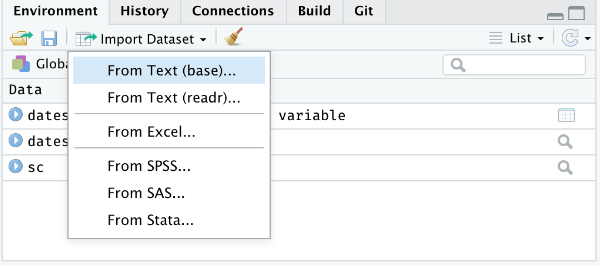
Importing data into R becomes time-intensive. The easiest way to import data into R is by using RStudio IDE. This feature can be accessed from the Environment pane or from the tools menu. The importers are grouped into three categories: Text data, Excel data, and statistical data. The details can be found here.

To access this feature, use the “Import Dataset” dropdown from the “Environment” pane:

Figure 1: Data Import RStudio Environment Pane

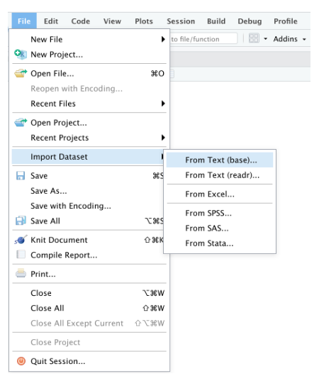
Or through the “File” menu, followed by the “Import Dataset” submenu:

Read Text File (.txt)

A text file is a type of computer file that contains only plain text — which means it includes letters, numbers, symbols, and spaces that can be read by humans and processed by computers. It doesn’t include any special formatting like bold, italics, or images—just raw text.

Key points about text files:

File extension: Usually ends in .txt
Editable with: Any text editor (like Notepad, TextEdit`, VS Code, etc.)
Encoding: Often uses encodings like ASCII or `UTF-8
Uses:
- Storing notes or data
- Writing code (before saving with a specific programming extension)
- Configuration files for software (like .ini, .conf, etc.)

Text files are often used for data storage and transfer because they are simple and widely supported. They can be easily created, edited, and read by both humans and machines. The easiest form of data to import into R is a simple text file. The primary function to import from a text file is read.table().

read.table(file, header = FALSE, sep = "", quote =""'",.....)

Code

# read .txt file
df.txt<-read.table(paste0(dataFolder,"test_data.txt"), header= TRUE)

Or you can directly load data directly from my Github data folder using following code:

Code

df.txt<-read.table("https://github.com/zia207/r-colab/raw/main/Data/R_Beginners/test_data.txt",
                    header= TRUE)
head(df.txt)

   ID treat  var rep    PH   TN   PN   GW ster   DTM   SW   GAs  STAs
1 Low    As BR01   1  84.0 28.3 27.7 35.7 20.5 126.0 28.4 0.762 14.60
2 Low    As BR01   2 111.7 34.0 30.0 58.1 14.8 119.0 36.7 0.722 10.77
3 Low    As BR01   3 102.3 27.7 24.0 44.6  5.8 119.7 32.9 0.858 12.69
4 Low    As BR06   1 118.0 23.3 19.7 46.4 20.3 119.0 40.0 1.053 18.23
5 Low    As BR06   2 115.3 16.7 12.3 19.9 32.3 120.0 28.2 1.130 13.72
6 Low    As BR06   3 111.0 19.0 15.3 35.9 14.9 116.3 42.3 1.011 15.97

Code

names(df.txt)

 [1] "ID"    "treat" "var"   "rep"   "PH"    "TN"    "PN"    "GW"    "ster" 
[10] "DTM"   "SW"    "GAs"   "STAs"

However, scan() function could be used to scan and read data. It is usually used to read data into vector or list or from file in R Language.

scan(scan(file = ““, what = double(), nmax = -1, n = -1, sep =”“,..)

Code

# Scan data 
#df.scan<-scan(paste0(dataFolder,"test_data.txt"),  what = list("", "", ""))   
df.scan<-scan("https://github.com/zia207/r-colab/raw/main/Data/R_Beginners/test_data.txt",
                    what = list("", "", ""))

Comma-Separated File (.csv)

A comma delimited or comma-separated file (CSV) is one where each value in the file is separated by a comma, although other characters can be used. Reading data from a CSV file is made easy by the read.csv(), an extension of read.table(). It facilitates the direct import of data from CSV files.

read.csv(file, header = TRUE, sep = ",", quote = """,...)

Code

df.csv<-read.csv(paste0(dataFolder,"test_data.csv"), header= TRUE)
head(df.csv)

  ID  treat  var rep    PH   TN   PN   GW ster   DTM   SW   GAs  STAs
1  1 Low As BR01   1  84.0 28.3 27.7 35.7 20.5 126.0 28.4 0.762 14.60
2  2 Low As BR01   2 111.7 34.0 30.0 58.1 14.8 119.0 36.7 0.722 10.77
3  3 Low As BR01   3 102.3 27.7 24.0 44.6  5.8 119.7 32.9 0.858 12.69
4  4 Low As BR06   1 118.0 23.3 19.7 46.4 20.3 119.0 40.0 1.053 18.23
5  5 Low As BR06   2 115.3 16.7 12.3 19.9 32.3 120.0 28.2 1.130 13.72
6  6 Low As BR06   3 111.0 19.0 15.3 35.9 14.9 116.3 42.3 1.011 15.97

Or you can load data directly from my Github data folder using following code:

Code

df.csv<-read.csv("https://github.com/zia207/r-colab/raw/main/Data/R_Beginners/test_data.csv",
                  header= TRUE)

Excel Files (.xlsx)

If you want to get data from Excel into R, one of the easiest ways to do it is to export the Excel file to a CSV file and then import it using the above method. But if you don’t want to do that, you can use the {readxl} package. It’s easy to use since it has no extra dependencies, so that you can install it on any operating system.

{readxl} package supports both the legacy .xls format and the modern xml-based .xlsx format. The libxls C library is used to support .xls, which abstracts away many of the complexities of the underlying binary format. To parse .xlsx, we use the RapidXML C++ library.

To install the package, you can use the following command:

install.packages(readxl")

read_excel() reads both xls and xlsx files and detects the format from the extension.

Code

# Import Sheet 1, from a excel file
df.xl <-readxl::read_excel(paste0(dataFolder,"test_data.xlsx"), 1) 
head(df.xl)

# A tibble: 6 × 13
     ID treat  var     rep    PH    TN    PN    GW  ster   DTM    SW   GAs  STAs
  <dbl> <chr>  <chr> <dbl> <dbl> <dbl> <dbl> <dbl> <dbl> <dbl> <dbl> <dbl> <dbl>
1     1 Low As BR01      1   84   28.3  27.7  35.7  20.5  126   28.4 0.762  14.6
2     2 Low As BR01      2  112.  34    30    58.1  14.8  119   36.7 0.722  10.8
3     3 Low As BR01      3  102.  27.7  24    44.6   5.8  120.  32.9 0.858  12.7
4     4 Low As BR06      1  118   23.3  19.7  46.4  20.3  119   40   1.05   18.2
5     5 Low As BR06      2  115.  16.7  12.3  19.9  32.3  120   28.2 1.13   13.7
6     6 Low As BR06      3  111   19    15.3  35.9  14.9  116.  42.3 1.01   16.0

JSON Files (.json)

JSON is an open standard file and lightweight data-interchange format that stands for JavaScript Object Notation. The JSON file is a text file that is language independent, self-describing, and easy to understand.

The JSON file is read by R as a list using the function fromJSON() of {rjson} package.

install.packages("rjson")
fromJSON(json_str, file, method = "C", unexpected.escape = "error", sim..)

Code

# read .json file
df.json <- rjson::fromJSON(file= paste0(dataFolder, "test_data.json"),  simplify=TRUE)
#print(df.json)

We can convert a JESON file to a regilar data frame:

Code

df.json <- as.data.frame(df.json)
head(df.json)

  ID  treat  var rep    PH   TN   PN   GW ster   DTM   SW   GAs  STAs
1  1 Low As BR01   1  84.0 28.3 27.7 35.7 20.5 126.0 28.4 0.762 14.60
2  2 Low As BR01   2 111.7 34.0 30.0 58.1 14.8 119.0 36.7 0.722 10.77
3  3 Low As BR01   3 102.3 27.7 24.0 44.6  5.8 119.7 32.9 0.858 12.69
4  4 Low As BR06   1 118.0 23.3 19.7 46.4 20.3 119.0 40.0 1.053 18.23
5  5 Low As BR06   2 115.3 16.7 12.3 19.9 32.3 120.0 28.2 1.130 13.72
6  6 Low As BR06   3 111.0 19.0 15.3 35.9 14.9 116.3 42.3 1.011 15.97

Import Data from Other Statistical Software

{foreign} packages is mostly used to read data stored by Minitab, SAS, SPSS, Stata, Systat, dBase, and so forth.

install.packages("foreign")

{Haven} enables R to read and write various data formats used by other statistical packages by wrapping with ReadStat C library. written b Haven is part of the tidyverse. Current it support SAS, SPSS and Stata files

install.packages("haven")

read.dta() function from {foreign} package can reads a file in Stata version 5-12 binary format (.dta) into a data frame.

Code

# read .dta file
df.dta_01 <- foreign::read.dta(paste0(dataFolder,"test_data.dta"))

read_dta() function from {haven} package can read a file in Stata version 5-12 binary format (.dta) into a data frame.

Code

# read .dta file
df.dta_02 <- haven::read_dta(paste0(dataFolder,"test_data.dta"))

SPSS File (.sav)

Foreign - read.spss()
Haven - read_sav()

Code

# read .sav file
df.sav_01 <- foreign::read.spss(paste0(dataFolder,"test_data.sav"))

Code

# read .sav file
df.sav_02 <- haven::read_sav(paste0(dataFolder,"test_data.sav")) 
#head(df.sav)

SAS File (.sas7bdat)

read_sas() function from haven package can read sas (.sas7bdat) file easily.

Code

# read .sas7bdat file
df.sas <- haven::read_sas(paste0(dataFolder,"test_data.sas7bdat")) 
#head(df.sas)

Export data from R

Data exporting is the process of saving data from R to a file format that can be used by other software or systems. This is important for sharing results, collaborating with others, or using the data in different applications. R provides several functions and packages to export data in various formats, including CSV, Excel, JSON, and more.

Write as CSV Files

First of all, let create a data frame that we will going to export as a text/CSV file.

Code

Variety =c("BR1","BR3", "BR16", "BR17", "BR18", "BR19","BR26",
          "BR27","BR28","BR29","BR35","BR36") # create a text vector
Yield = c(5.2,6.0,6.6,5.6,4.7,5.2,5.7,
                5.9,5.3,6.8,6.2,5.8) # create numerical vector
rice.data= data.frame(Variety, Yield)
head(rice.data)

  Variety Yield
1     BR1   5.2
2     BR3   6.0
3    BR16   6.6
4    BR17   5.6
5    BR18   4.7
6    BR19   5.2

The popular R base functions for writing data are write.table(), write.csv(), write.csv2() and write.delim() functions.

Before start, you need to specify the working or destination directory in where you will save the data.

Code

write.csv(rice.data, paste0(dataFolder, "rice_data.csv"), row.names = F) # no row names

Write as Excel File

Exporting data from R to Excel can be achieved with several packages. The most known package to export data frames or tables as Excel is “writexl”, that provides the write_xlsx functions.

Code

# write as xlsx file
writexl::write_xlsx(rice.data, paste0(dataFolder, "rice_data.xlsx"))

JSON Objects

To write JSON Object to file, the toJSON() function from the rjson library can be used to prepare a JSON object and then use the write() function for writing the JSON object to a local file.

Code

# create a JSON object
jsonData <-rjson::toJSON(rice.data)
# write JSON objects
write(jsonData, file= paste0(dataFolder,"rice_data.json"))

R Data File

If you want to share the data from R as Objects and share those with your colleagues through different systems so that they can use it right away into their R-workspace. These objects are of two types .rda/.RData which can be used to store some or all objects, functions from R global environment.

The save() function allows us to save multiple objects into our global environment:

Note

If you specify save.image(file = "R_objects.RData") Export all objects (the workspace image).

To save only one object it is more recommended saving it as RDS with the saveRDS() function:

Code

# write .RDS file
saveRDS(rice.data,  file= paste0(dataFolder,"rice_data.rds"))

Note

If you specify compress = TRUE*as argument of the above functions the file will be compressed by default as gzip.

Export to Other Statistcal Software

STATA File

If you want export data from R to STATA, you will need to use the write.dta() function of the {foreign} package.

Code

# write dta file
foreign::write.dta(rice.data, file= paste0(dataFolder,"rice_data.dta"))

SPSS File

Haven enables R to read and write various data formats used by other statistical packages by wrapping with ReadStat C library. written b Haven is part of the tidyverse. Current it support SAS, SPSS and Stata files

The write_sav() function of {haven} package can be used to export R-object to SPSS

Code

# write .sav file
haven::write_sav(rice.data, "/home/zia207/Dropbox/R_Website/R_Beginner/Data/rice_data.sav")

SAS File

The write_sas() function of {haven} package can be used to export R-object to SAS (.sas7bdat)

Code

# write .sav file
haven::write_sas(rice.data, "/home/zia207/Dropbox/R_Website/R_Beginner/Data/rice_data.sas7bdat")

Summary and Conclusion

This guide covers the necessary skills to import and export data into/from R for data analysis or statistical modeling. It discusses various data formats, including CSV, Excel, and text files, and strategies for managing missing values, data types, and potential import challenges. Advanced import/export techniques are also covered, allowing you to streamline your workflow and spend more time analyzing data. By practicing these techniques, you can transform your analysis into actionable insights and make a meaningful impact in your field.

Data Import/Export to/from R

Introduction

Check and Install Required R Packages

Verify Installation

Load R-packages

Loaded Packages

Data

Data Import Into R

Importing data using R-Studio IDE

Read Text File (.txt)

Comma-Separated File (.csv)

Excel Files (.xlsx)

JSON Files (.json)

Import Data from Other Statistical Software

STATA File (.dta)

SPSS File (.sav)

SAS File (.sas7bdat)

Export data from R

Write as CSV Files

Write as Excel File

JSON Objects

R Data File

Export to Other Statistcal Software

STATA File

SPSS File

SAS File

Summary and Conclusion

References