Multiple Regression Analysis in R

This tutorial is designed to provide a comprehensive introduction to Multiple Linear Regression (MLR) using R, a powerful statistical programming language. MLR is a widely used statistical technique that allows researchers and analysts to model the relationship between a dependent variable and multiple independent variables. This tutorial will guide you through the fundamental concepts of MLR, its applications, and practical implementation in R.

Introduction

Multiple Regression Analysis is a statistical method used to examine the relationship between a dependent variable and two or more independent variables. It extends the concept of simple linear regression, which involves studying the relationship between a dependent variable and a single independent variable. In multiple regression, the goal is to understand how multiple independent variables together influence the variation in the dependent variable.

Suppose you have a dataset with \(n\) observations and \(k\) independent variables. The matrix notation for the multiple linear regression model is as follows:

1. Matrix of Independent Variables (Design Matrix):

   • Let \(X\) be the design matrix, which has dimensions \(n \times (k+1)\).
   • The first column of \(X\) is usually a column of ones, representing the intercept term.
   • The remaining columns correspond to the values of the independent variables for each observation.

\[ X = \begin{bmatrix} 1 & x_{11} & x_{12} & \ldots & x_{1k} \\ 1 & x_{21} & x_{22} & \ldots & x_{2k} \\ \vdots & \vdots & \vdots & \ddots & \vdots \\ 1 & x_{n1} & x_{n2} & \ldots & x_{nk} \end{bmatrix} \]

2. Vector of Coefficients:

   • Let \(\beta\) be the vector of coefficients, with dimensions \((k+1) \times 1\).
   • The elements of \(\beta\) represent the intercept and the coefficients for the independent variables.

\[ \beta = \begin{bmatrix} \beta_0 \\ \beta_1 \\ \beta_2 \\ \vdots \\ \beta_k \end{bmatrix} \]

3. Vector of Dependent Variables:

   • Let \(Y\) be the vector of dependent variables, with dimensions \(n \times 1\).
   • Each element of \(Y\) corresponds to the dependent variable for each observation.

\[ Y = \begin{bmatrix} y_1 \\ y_2 \\ \vdots \\ y_n \end{bmatrix}\]

4. Error Vector:

   • Let \(\varepsilon\) be the vector of errors (residuals), with dimensions \(n \times 1\).
   • Each element of \(\varepsilon\) represents the difference between the observed and predicted values.

   \[ \varepsilon = \begin{bmatrix} \varepsilon_1 \\ \varepsilon_2 \\ \vdots \\ \varepsilon_n \end{bmatrix} \]

Now, the multiple linear regression model can be expressed in matrix notation as:

\[ Y = X\beta + \varepsilon \]

This equation captures the relationship between the dependent variable \(Y\), the design matrix \(X\), the coefficient vector \(\beta\), and the error vector (\(\varepsilon\)). The goal of regression analysis is to estimate the values of the coefficients in () that minimize the sum of squared errors (least squares method). This estimation can be expressed in matrix form as:

\[ \hat{\beta} = (X^TX)^{-1}X^TY \]

where \(\hat{\beta}\) represents the estimated coefficients. Matrix notation provides a concise and efficient way to represent and solve regression problems, especially when dealing with multiple variables.

Multiple Linear Regression Analysis from Scratch

Here’s how to perform multiple regression from scratch in R with four predictors, including summary statistics and R² values:

set.seed(123)  # For reproducibility

# Generate sample data
n <- 100       # Number of observations
X <- matrix(rnorm(n * 4), ncol = 4)
colnames(X) <- c("X1", "X2", "X3", "X4")
true_beta <- c(2, 3, -1, 0.5, 2)  # True coefficients (intercept first)
X_with_intercept <- cbind(1, X)     # Design matrix with intercept
error <- rnorm(n, sd = 2)
y <- X_with_intercept %*% true_beta + error

# Calculate coefficients using normal equation
XTX <- t(X_with_intercept) %*% X_with_intercept
beta_hat <- solve(XTX) %*% t(X_with_intercept) %*% y

# Calculate residuals and R-squared
y_hat <- X_with_intercept %*% beta_hat
residuals <- y - y_hat
SS_residual <- sum(residuals^2)
SS_total <- sum((y - mean(y))^2)
R_squared <- 1 - (SS_residual / SS_total)

# Calculate standard errors and p-values
df <- n - length(beta_hat)          # Degrees of freedom
sigma_sq_hat <- SS_residual / df    # Residual variance estimate
var_cov <- sigma_sq_hat * solve(XTX) # Variance-covariance matrix
se <- sqrt(diag(var_cov))           # Standard errors
t_values <- beta_hat / se           # t-statistics
p_values <- 2 * pt(abs(t_values), df = df, lower.tail = FALSE)  # p-values

# Create summary table
summary_df <- data.frame(
  Estimate = round(beta_hat, 4),
  Std.Error = round(se, 4),
  t.value = round(t_values, 4),
  p.value = ifelse(p_values < 0.001, "<0.001", round(p_values, 4))
)

rownames(summary_df) <- c("(Intercept)", colnames(X))

# Display results
cat("Multiple Regression Results from Scratch\n")

Multiple Regression Results from Scratch

cat("========================================\n")

========================================

print(summary_df)

            Estimate Std.Error t.value p.value
(Intercept)   2.2323    0.2000 11.1616  <0.001
X1            2.5515    0.2180 11.7055  <0.001
X2           -1.2830    0.2041 -6.2867  <0.001
X3            0.3991    0.2094  1.9063  0.0596
X4            1.9533    0.1901 10.2741  <0.001

cat("\nResidual standard error:", round(sqrt(sigma_sq_hat), 3), "on", df, "degrees of freedom\n")

Residual standard error: 1.959 on 95 degrees of freedom

cat("Multiple R-squared: ", round(R_squared, 4), "\n")

Multiple R-squared:  0.7413 

Multiple Linear Regression Analysis in R

In this sectiomn, we will explore how to perform MLR in R, interpret the results, and visualize the findings. We will also cover important concepts such as model diagnostics, performance evaluation, and relative importance of predictors.

Check and Install Required Packages

packages <- c('tidyverse', 
         'broom',
         'report', 
         'stargazer',
         'performance',
         'jtools',
         'relaimpo',
         'ggpmisc',
         'see',
         'Metrics'
           )

# Install missing packages
new_packages <- packages[!(packages %in% installed.packages()[,"Package"])]
if(length(new_packages)) install.packages(new_packages)

Verify Installation

# Verify installation
cat("Installed packages:\n")

Installed packages:

print(sapply(packages, requireNamespace, quietly = TRUE))

Registered S3 methods overwritten by 'ggpp':
  method                  from   
  heightDetails.titleGrob ggplot2
  widthDetails.titleGrob  ggplot2

  tidyverse       broom      report   stargazer performance      jtools 
       TRUE        TRUE        TRUE        TRUE        TRUE        TRUE 
   relaimpo     ggpmisc         see     Metrics 
       TRUE        TRUE        TRUE        TRUE 

Load Packages

# Load packages with suppressed messages
invisible(lapply(packages, function(pkg) {
  suppressPackageStartupMessages(library(pkg, character.only = TRUE))
}))

Check Loaded Packages

# Check loaded packages
cat("Successfully loaded packages:\n")

Successfully loaded packages:

print(search()[grepl("package:", search())])

 [1] "package:Metrics"     "package:see"         "package:ggpmisc"    
 [4] "package:ggpp"        "package:relaimpo"    "package:mitools"    
 [7] "package:survey"      "package:survival"    "package:Matrix"     
[10] "package:grid"        "package:boot"        "package:MASS"       
[13] "package:jtools"      "package:performance" "package:stargazer"  
[16] "package:report"      "package:broom"       "package:lubridate"  
[19] "package:forcats"     "package:stringr"     "package:dplyr"      
[22] "package:purrr"       "package:readr"       "package:tidyr"      
[25] "package:tibble"      "package:ggplot2"     "package:tidyverse"  
[28] "package:stats"       "package:graphics"    "package:grDevices"  
[31] "package:utils"       "package:datasets"    "package:methods"    
[34] "package:base"       

Data

All data set use in this exercise can be downloaded from my Dropbox or from my Github accounts.

We will use read_csv() function of readr package to import data as a tidy data.

# Load data
mf<-read_csv("https://github.com/zia207/r-colab/raw/main/Data/Regression_analysis/gp_soil_data.csv")

Fit a MLR model with continuous predictors

We aim to create a multiple regression model that incorporates various predictors, such as DEM (Digital Elevation Model), Slope, TPI (Topographic Position Index), MAT (Mean Annual Temperature), MAP (Mean Annual Precipitation), and NDVI (Normalized Difference Vegetation Index). Our objective is to uncover the factors that affect the levels of soil organic carbon and enhance our comprehension of the underlying mechanisms.

# Create a data-frame
df<-mf  |>  
    dplyr::select(SOC, DEM, Slope, MAT, MAP,NDVI)

# fit a MLR model
mlr_01<-lm(SOC~DEM+Slope+MAT+MAP+NDVI, df)
summary(mlr_01)

Call:
lm(formula = SOC ~ DEM + Slope + MAT + MAP + NDVI, data = df)

Residuals:
     Min       1Q   Median       3Q      Max 
-13.5216  -2.1087  -0.4608   1.3395  16.3788 

Coefficients:
              Estimate Std. Error t value Pr(>|t|)    
(Intercept)  2.2088309  1.8002202   1.227 0.220457    
DEM         -0.0003853  0.0005465  -0.705 0.481201    
Slope        0.1660845  0.0632881   2.624 0.008972 ** 
MAT         -0.3239459  0.0821817  -3.942 9.34e-05 ***
MAP          0.0061026  0.0016366   3.729 0.000216 ***
NDVI         8.6687410  2.0697085   4.188 3.37e-05 ***
---
Signif. codes:  0 '***' 0.001 '**' 0.01 '*' 0.05 '.' 0.1 ' ' 1

Residual standard error: 3.812 on 461 degrees of freedom
Multiple R-squared:  0.4354,    Adjusted R-squared:  0.4293 
F-statistic: 71.09 on 5 and 461 DF,  p-value: < 2.2e-16

Create a Regression Summary Table

We can create a regression summary table with tidy() function from the broom and stargazer() function from stargazer packages.

#library(broom)
broom::tidy(mlr_01)

# A tibble: 6 × 5
  term         estimate std.error statistic   p.value
  <chr>           <dbl>     <dbl>     <dbl>     <dbl>
1 (Intercept)  2.21      1.80         1.23  0.220    
2 DEM         -0.000385  0.000547    -0.705 0.481    
3 Slope        0.166     0.0633       2.62  0.00897  
4 MAT         -0.324     0.0822      -3.94  0.0000934
5 MAP          0.00610   0.00164      3.73  0.000216 
6 NDVI         8.67      2.07         4.19  0.0000337

#library(stargazer)
stargazer::stargazer(mlr_01,type="text")

===============================================
                        Dependent variable:    
                    ---------------------------
                                SOC            
-----------------------------------------------
DEM                           -0.0004          
                              (0.001)          
                                               
Slope                        0.166***          
                              (0.063)          
                                               
MAT                          -0.324***         
                              (0.082)          
                                               
MAP                          0.006***          
                              (0.002)          
                                               
NDVI                         8.669***          
                              (2.070)          
                                               
Constant                       2.209           
                              (1.800)          
                                               
-----------------------------------------------
Observations                    467            
R2                             0.435           
Adjusted R2                    0.429           
Residual Std. Error      3.812 (df = 461)      
F Statistic           71.094*** (df = 5; 461)  
===============================================
Note:               *p<0.1; **p<0.05; ***p<0.01

Genrate Report

We can generate report for linear model using report() function of report package:

install.package(“report”)

#library(report)
report::report(mlr_01)

We fitted a linear model (estimated using OLS) to predict SOC with DEM, Slope,
MAT, MAP and NDVI (formula: SOC ~ DEM + Slope + MAT + MAP + NDVI). The model
explains a statistically significant and substantial proportion of variance (R2
= 0.44, F(5, 461) = 71.09, p < .001, adj. R2 = 0.43). The model's intercept,
corresponding to DEM = 0, Slope = 0, MAT = 0, MAP = 0 and NDVI = 0, is at 2.21
(95% CI [-1.33, 5.75], t(461) = 1.23, p = 0.220). Within this model:

  - The effect of DEM is statistically non-significant and negative (beta =
-3.85e-04, 95% CI [-1.46e-03, 6.89e-04], t(461) = -0.70, p = 0.481; Std. beta =
-0.06, 95% CI [-0.22, 0.11])
  - The effect of Slope is statistically significant and positive (beta = 0.17,
95% CI [0.04, 0.29], t(461) = 2.62, p = 0.009; Std. beta = 0.15, 95% CI [0.04,
0.27])
  - The effect of MAT is statistically significant and negative (beta = -0.32,
95% CI [-0.49, -0.16], t(461) = -3.94, p < .001; Std. beta = -0.26, 95% CI
[-0.39, -0.13])
  - The effect of MAP is statistically significant and positive (beta = 6.10e-03,
95% CI [2.89e-03, 9.32e-03], t(461) = 3.73, p < .001; Std. beta = 0.25, 95% CI
[0.12, 0.38])
  - The effect of NDVI is statistically significant and positive (beta = 8.67,
95% CI [4.60, 12.74], t(461) = 4.19, p < .001; Std. beta = 0.28, 95% CI [0.15,
0.41])

Standardized parameters were obtained by fitting the model on a standardized
version of the dataset. 95% Confidence Intervals (CIs) and p-values were
computed using a Wald t-distribution approximation.

Model Performance

#library(performance)
performance::model_performance(mlr_01)

# Indices of model performance

AIC      |     AICc |      BIC |    R2 | R2 (adj.) |  RMSE | Sigma
------------------------------------------------------------------
2583.012 | 2583.256 | 2612.037 | 0.435 |     0.429 | 3.787 | 3.812

Comprehensive visualization of model checks

performance::check_model(mlr_01)

Fit a MLR Model with continous and catagorical predictors

Now we will update the MLR model by adding tow categorical variables: NLCD (National Land Cover Database), and FRG (Forest Regimes)

# Create a data-frame
df_02<-mf %>% dplyr::select(SOC, DEM, Slope, MAT, MAP,NDVI, NLCD, FRG)
# fit MLR model
mlr_02<-lm(SOC~DEM+Slope+MAT+MAP+NDVI+NLCD+FRG, df_02)

stargazer::stargazer(mlr_02,type="text")

====================================================
                             Dependent variable:    
                         ---------------------------
                                     SOC            
----------------------------------------------------
DEM                                -0.0004          
                                   (0.001)          
                                                    
Slope                              0.155**          
                                   (0.069)          
                                                    
MAT                               -0.400***         
                                   (0.101)          
                                                    
MAP                               0.007***          
                                   (0.002)          
                                                    
NDVI                              6.828***          
                                   (2.452)          
                                                    
NLCDHerbaceous                     -1.468*          
                                   (0.880)          
                                                    
NLCDPlanted/Cultivated             -1.698*          
                                   (0.990)          
                                                    
NLCDShrubland                      -1.161           
                                   (0.798)          
                                                    
FRGFire Regime Group II           2.897***          
                                   (1.038)          
                                                    
FRGFire Regime Group III            1.582           
                                   (1.001)          
                                                    
FRGFire Regime Group IV             1.131           
                                   (1.134)          
                                                    
FRGFire Regime Group V              0.957           
                                   (1.391)          
                                                    
FRGIndeterminate FRG                1.789           
                                   (1.739)          
                                                    
Constant                            2.529           
                                   (2.832)          
                                                    
----------------------------------------------------
Observations                         467            
R2                                  0.451           
Adjusted R2                         0.436           
Residual Std. Error           3.790 (df = 453)      
F Statistic               28.669*** (df = 13; 453)  
====================================================
Note:                    *p<0.1; **p<0.05; ***p<0.01

Generate Report

report::report(mlr_02)

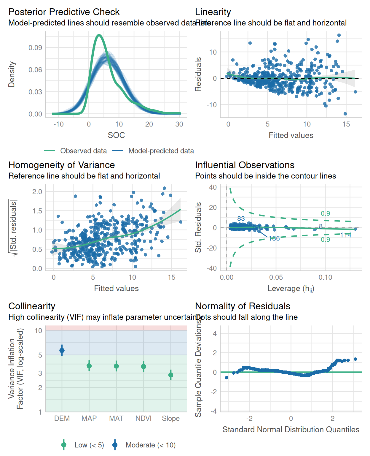
We fitted a linear model (estimated using OLS) to predict SOC with DEM, Slope,
MAT, MAP, NDVI, NLCD and FRG (formula: SOC ~ DEM + Slope + MAT + MAP + NDVI +
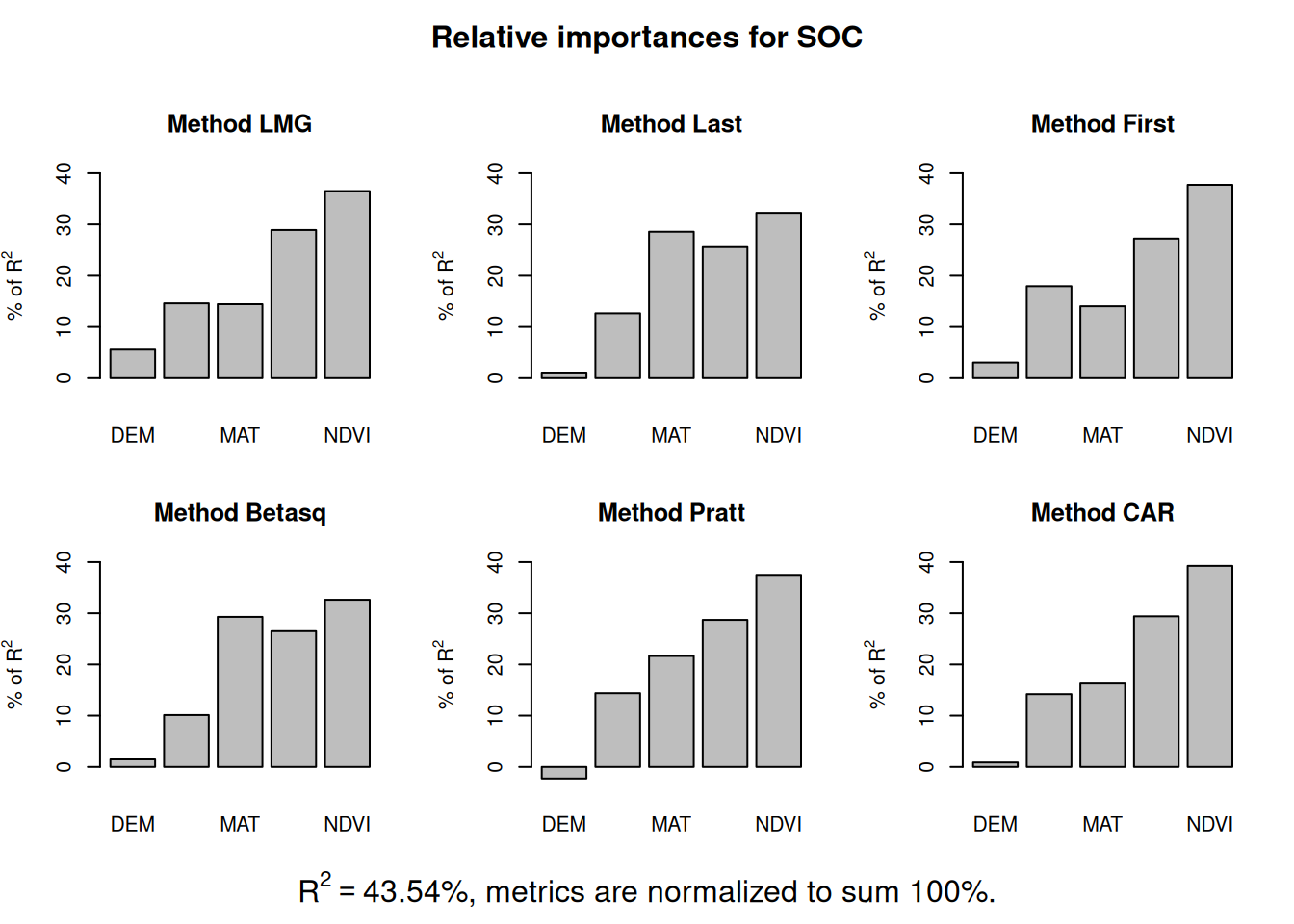
NLCD + FRG). The model explains a statistically significant and substantial
proportion of variance (R2 = 0.45, F(13, 453) = 28.67, p < .001, adj. R2 =
0.44). The model's intercept, corresponding to DEM = 0, Slope = 0, MAT = 0, MAP
= 0, NDVI = 0, NLCD = Forest and FRG = Fire Regime Group I, is at 2.53 (95% CI
[-3.04, 8.09], t(453) = 0.89, p = 0.372). Within this model:

  - The effect of DEM is statistically non-significant and negative (beta =
-4.48e-04, 95% CI [-1.79e-03, 8.92e-04], t(453) = -0.66, p = 0.511; Std. beta =
-0.07, 95% CI [-0.27, 0.14])
  - The effect of Slope is statistically significant and positive (beta = 0.16,
95% CI [0.02, 0.29], t(453) = 2.27, p = 0.024; Std. beta = 0.14, 95% CI [0.02,
0.27])
  - The effect of MAT is statistically significant and negative (beta = -0.40,
95% CI [-0.60, -0.20], t(453) = -3.98, p < .001; Std. beta = -0.33, 95% CI
[-0.49, -0.16])
  - The effect of MAP is statistically significant and positive (beta = 6.76e-03,
95% CI [3.26e-03, 0.01], t(453) = 3.80, p < .001; Std. beta = 0.28, 95% CI
[0.13, 0.42])
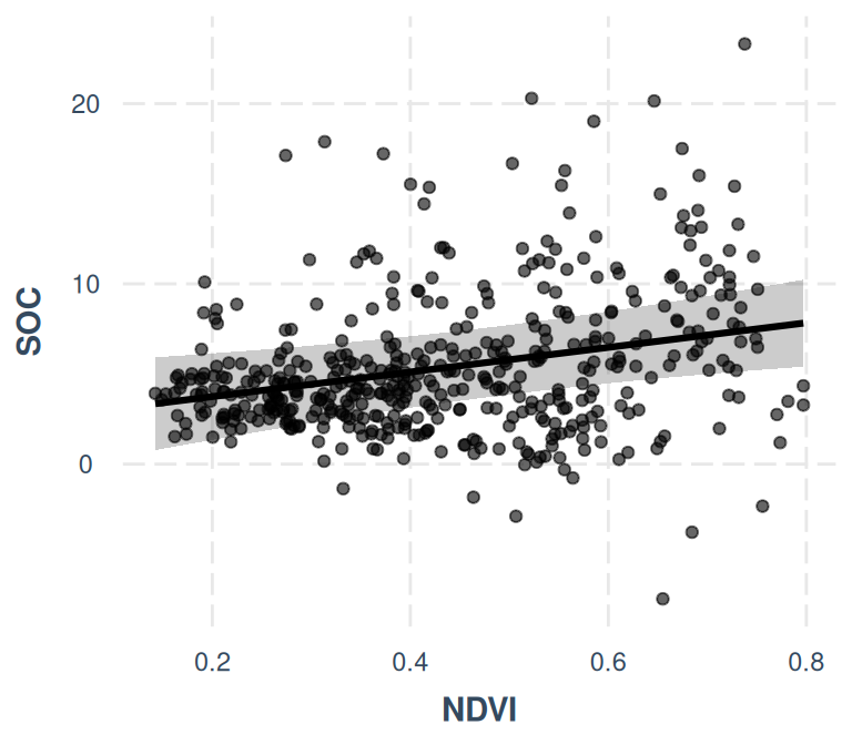
  - The effect of NDVI is statistically significant and positive (beta = 6.83,
95% CI [2.01, 11.65], t(453) = 2.78, p = 0.006; Std. beta = 0.22, 95% CI [0.06,
0.37])
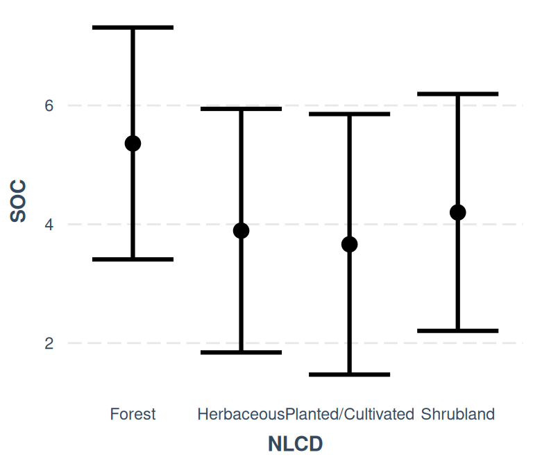
  - The effect of NLCD [Herbaceous] is statistically non-significant and negative
(beta = -1.47, 95% CI [-3.20, 0.26], t(453) = -1.67, p = 0.096; Std. beta =
-0.29, 95% CI [-0.63, 0.05])
  - The effect of NLCD [Planted/Cultivated] is statistically non-significant and
negative (beta = -1.70, 95% CI [-3.64, 0.25], t(453) = -1.72, p = 0.087; Std.
beta = -0.34, 95% CI [-0.72, 0.05])
  - The effect of NLCD [Shrubland] is statistically non-significant and negative
(beta = -1.16, 95% CI [-2.73, 0.41], t(453) = -1.46, p = 0.146; Std. beta =
-0.23, 95% CI [-0.54, 0.08])
  - The effect of FRG [Fire Regime Group II] is statistically significant and
positive (beta = 2.90, 95% CI [0.86, 4.94], t(453) = 2.79, p = 0.005; Std. beta
= 0.57, 95% CI [0.17, 0.98])
  - The effect of FRG [Fire Regime Group III] is statistically non-significant
and positive (beta = 1.58, 95% CI [-0.39, 3.55], t(453) = 1.58, p = 0.115; Std.
beta = 0.31, 95% CI [-0.08, 0.70])
  - The effect of FRG [Fire Regime Group IV] is statistically non-significant and
positive (beta = 1.13, 95% CI [-1.10, 3.36], t(453) = 1.00, p = 0.319; Std.
beta = 0.22, 95% CI [-0.22, 0.67])
  - The effect of FRG [Fire Regime Group V] is statistically non-significant and
positive (beta = 0.96, 95% CI [-1.78, 3.69], t(453) = 0.69, p = 0.492; Std.
beta = 0.19, 95% CI [-0.35, 0.73])
  - The effect of FRG [Indeterminate FRG] is statistically non-significant and
positive (beta = 1.79, 95% CI [-1.63, 5.21], t(453) = 1.03, p = 0.304; Std.
beta = 0.35, 95% CI [-0.32, 1.03])

Standardized parameters were obtained by fitting the model on a standardized
version of the dataset. 95% Confidence Intervals (CIs) and p-values were
computed using a Wald t-distribution approximation.

Model Performance

performance::model_performance(mlr_02)

# Indices of model performance

AIC      |     AICc |      BIC |    R2 | R2 (adj.) |  RMSE | Sigma
------------------------------------------------------------------
2585.591 | 2586.655 | 2647.786 | 0.451 |     0.436 | 3.733 | 3.790

Models comparison

The compare_performance() function can be used to compare the performance and quality of several models (including models of different types). We can easily compute and a composite index of model performance and sort the models from the best one to the worse.

performance::compare_performance(mlr_01, mlr_02, rank = TRUE)

# Comparison of Model Performance Indices

Name   | Model |    R2 | R2 (adj.) |  RMSE | Sigma | AIC weights | AICc weights
-------------------------------------------------------------------------------
mlr_02 |    lm | 0.451 |     0.436 | 3.733 | 3.790 |       0.216 |        0.155
mlr_01 |    lm | 0.435 |     0.429 | 3.787 | 3.812 |       0.784 |        0.845

Name   | BIC weights | Performance-Score
----------------------------------------
mlr_02 |    1.73e-08 |            57.14%
mlr_01 |       1.000 |            42.86%

Visualisation of indices of models’ performance

Finally, we provide convenient visualization (the see package must be installed).

#| warning: false
#| error: false

#| fig.width: 4
#| fig.height: 4

plot(compare_performance(mlr_01, mlr_02, rank = TRUE))

Testing models

test_performance() and test_bf, carries out the most relevant and appropriate tests based on the input (for instance, whether the models are nested or not).

performance::test_performance(mlr_01, mlr_02)

Name   | Model |      BF | df | df_diff |  Chi2 |     p
-------------------------------------------------------
mlr_01 |    lm |         |  7 |         |       |      
mlr_02 |    lm | < 0.001 | 15 |    8.00 | 13.42 | 0.098
Models were detected as nested (in terms of fixed parameters) and are compared in sequential order.

#test_bf(mlr_01, mlr_02)

Regression Model visualization by jtools

Th “jtools” package consists of a series of functions to automate visualization regression model.

install.packages (“jtools”)

Console regression summaries

summ() is a replacement for summary() that provides the user several options for formatting regression summaries. It supports glm, svyglm, and merMod objects as input as well. It supports calculation and reporting of robust standard errors via the sandwich package.

jtools::summ(mlr_02)

Observations	467
Dependent variable	SOC
Type	OLS linear regression

F(13,453)	28.67
R²	0.45
Adj. R²	0.44

	Est.	S.E.	t val.	p
(Intercept)	2.53	2.83	0.89	0.37
DEM	-0.00	0.00	-0.66	0.51
Slope	0.16	0.07	2.27	0.02
MAT	-0.40	0.10	-3.98	0.00
MAP	0.01	0.00	3.80	0.00
NDVI	6.83	2.45	2.78	0.01
NLCDHerbaceous	-1.47	0.88	-1.67	0.10
NLCDPlanted/Cultivated	-1.70	0.99	-1.72	0.09
NLCDShrubland	-1.16	0.80	-1.46	0.15
FRGFire Regime Group II	2.90	1.04	2.79	0.01
FRGFire Regime Group III	1.58	1.00	1.58	0.11
FRGFire Regime Group IV	1.13	1.13	1.00	0.32
FRGFire Regime Group V	0.96	1.39	0.69	0.49
FRGIndeterminate FRG	1.79	1.74	1.03	0.30
Standard errors: OLS

You can also get variance inflation factors (VIFs) and partial/semipartial (AKA part) correlations. Partial correlations are only available for OLS models. You may also substitute confidence intervals in place of standard errors and you can choose whether to show p values.

jtools::summ(mlr_02, 
     scale = TRUE,
     vifs = TRUE, 
     part.corr = TRUE, 
     confint = TRUE, 
     pvals = FALSE)

Observations	467
Dependent variable	SOC
Type	OLS linear regression

F(13,453)	28.67
R²	0.45
Adj. R²	0.44

	Est.	2.5%	97.5%	t val.	VIF	partial.r	part.r
(Intercept)	5.36	3.41	7.31	5.40	NA	NA	NA
DEM	-0.34	-1.38	0.69	-0.66	8.94	-0.03	-0.02
Slope	0.73	0.10	1.36	2.27	3.37	0.11	0.08
MAT	-1.64	-2.45	-0.83	-3.98	5.53	-0.18	-0.14
MAP	1.40	0.68	2.12	3.80	4.40	0.18	0.13
NDVI	1.11	0.33	1.89	2.78	5.11	0.13	0.10
NLCDHerbaceous	-1.47	-3.20	0.26	-1.67	9.63	-0.08	-0.06
NLCDPlanted/Cultivated	-1.70	-3.64	0.25	-1.72	9.63	-0.08	-0.06
NLCDShrubland	-1.16	-2.73	0.41	-1.46	9.63	-0.07	-0.05
FRGFire Regime Group II	2.90	0.86	4.94	2.79	8.60	0.13	0.10
FRGFire Regime Group III	1.58	-0.39	3.55	1.58	8.60	0.07	0.05
FRGFire Regime Group IV	1.13	-1.10	3.36	1.00	8.60	0.05	0.03
FRGFire Regime Group V	0.96	-1.78	3.69	0.69	8.60	0.03	0.02
FRGIndeterminate FRG	1.79	-1.63	5.21	1.03	8.60	0.05	0.04
Standard errors: OLS; Continuous predictors are mean-centered and scaled by 1 s.d. The outcome variable remains in its original units.

Note

Variance Inflation factors (VIFs): Variance inflation factors (VIFs) are a measure of multicollinearity in regression analysis. Multicollinearity occurs when two or more independent variables in a regression model are highly correlated, which can lead to unreliable estimates of the regression coefficients.

VIF is calculated for each independent variable in the regression model, and it represents the extent to which that variable’s variance is inflated by the presence of other independent variables in the model. Specifically, VIF measures the ratio of the variance of the coefficient estimate for a particular independent variable in a model that includes all the independent variables, to the variance of the coefficient estimate for that same variable in a model that includes only that variable and the constant.

A VIF of 1 indicates that there is no multicollinearity between the independent variable and the other variables in the model. Generally, a VIF greater than 5 or 10 is considered high, indicating that multicollinearity is a potential issue.

Partial/semipartial (AKA part) correlations: Partial or semipartial (also known as part) correlations are a statistical technique used to determine the degree of association between two variables while controlling for the effects of one or more additional variables.

Partial correlations measure the association between two variables, while controlling for the effects of other variables in the analysis. It calculates the correlation coefficient between two variables while holding all other variables constant. Partial correlation is used to determine the unique contribution of each variable in the relationship between two other variables.

Semipartial correlations, on the other hand, measure the degree of association between two variables while controlling for the effects of one additional variable. It is also known as a part correlation, as it quantifies the unique variance that a particular independent variable explains in the dependent variable, after controlling for the other independent variables in the analysis.

Partial and semipartial correlations are useful in situations where two or more variables are highly correlated, and it is difficult to determine their individual effects on the dependent variable. By controlling for the effects of other variables, these correlations can provide a more accurate estimate of the strength of the relationship between two variables. They are commonly used in regression analysis, where the goal is to determine the unique contribution of each independent variable in predicting the dependent variable.

Plotting model predictions (effect_plot())

Sometimes, the best way to understand your model is to look at the prediction performance. Rather than look at coefficients, effect_plot() lets you plot predictions across values of a predictor variable alongside the observed data.

# Effect of a continuous variable
jtools::effect_plot(mlr_02, pred = NDVI, interval = TRUE,  partial.residuals = TRUE)

# Effect of a categorical variable
jtools::effect_plot(mlr_02, pred =NLCD, interval = TRUE)

Relative Importance

The relaimpo package provides measures of relative importance for each of the predictors in the model. See help(calc.relimp) for details on the four measures of relative importance provided.

install.package(“relaimpo”)

#| fig.width: 8
#| fig.height: 8

# Calculate Relative Importance for Each Predictor
#library(relaimpo)
rvip<-relaimpo::calc.relimp(mlr_01,
                 type = c("lmg", "last", "first", "betasq", "pratt", "car"),
                 rela=TRUE)
plot(rvip)

Note

lmg: is the R2 contribution averaged over orderings among regressors, cf. e.g. Lindeman, Merenda and Gold 1980, p.119ff or Chevan and Sutherland (1991).

pmvd: is the proportional marginal variance decomposition as proposed by Feldman (2005) (non-US version only). It can be interpreted as a weighted average over orderings among regressors, with data-dependent weights.

last: is each variables contribution when included last, also sometimes called usefulness.

first: is each variables contribution when included first, which is just the squared covariance between y and the variable.

betasq: is the squared standardized coefficient.

pratt: is the product of the standardized coefficient and the correlation.

genizi: is the \(R^2\) decomposition according to Genizi 1993

car: is the R2 decomposition according to Zuber and Strimmer 2010, also available from package care (squares of scores produced by function carscore

Summary and Conclusion

This tutorial has provided a comprehensive overview of Multiple Linear Regression using R, a powerful statistical tool for modeling relationships between multiple variables. We started by understanding the fundamental concepts, explored data preparation techniques, and delved into model building and evaluation. By utilizing the lm() function in R, we created MLR models and interpreted the coefficients to gain insights into the impact of each predictor variable on the response variable. Additionally, diagnostic plots and statistical tests were employed to validate the model assumptions and ensure the reliability of our results.

It is crucial to recognize the significance of Multiple Linear Regression in various fields, from finance and economics to social sciences and beyond. MLR equips us with the ability to make informed predictions and understand the complex interplay between different factors that influence an outcome. As you embark on your journey with MLR, consider exploring advanced topics such as feature engineering, interaction terms, and model regularization to enhance the predictive power of your models. Continuously honing your model interpretation and validation skills will contribute to more accurate and reliable predictions in real-world scenarios. This tutorial serves as a solid foundation, but the realm of Multiple Linear Regression is vast and ever-evolving. Embrace the knowledge gained here and apply it to your datasets, uncovering patterns and relationships that drive meaningful insights.

References

1. Multiple Linear Regression

2. report

3. performance

4. jtools