Correlation Analysis with R

This section is designed to provide a comprehensive introduction to correlation analysis using R. Correlation analysis is a fundamental statistical technique used to assess the strength and direction of the relationship between two or more variables. It plays a crucial role in various fields, including social sciences, finance, healthcare, and environmental studies. By the end of this tutorial, you will have a solid understanding of conducting correlation analysis in R. This will enable you to effectively explore relationships within your datasets and draw meaningful insights from your data.

Introduction

Correlation is a statistical technique used to measure the degree of association between two continuous variables. It measures the linear relationship between two variables, indicating how closely they are related. A correlation coefficient ranges from -1 to +1, with a value of -1 indicating a perfect negative correlation, 0 indicating no correlation, and +1 indicating a perfect positive correlation. Correlation analysis is commonly used in many fields, including economics, finance, psychology, and social sciences, to help understand the relationship between variables and to make predictions based on that relationship.

The most common correlation coefficient is the Pearson correlation coefficient (denoted by \(r\)), and the formula is as follows:

\[ r = \frac{\sum_{i=1}^{n} (X_i - \bar{X})(Y_i - \bar{Y})}{\sqrt{\sum_{i=1}^{n} (X_i - \bar{X})^2 \sum_{i=1}^{n} (Y_i - \bar{Y})^2}} \]

Where: -

\(r\) is the Pearson correlation coefficient.

- \(X_i\) and \(Y_i\) are the individual data points for the two variables.

\(\bar{X}\) and \(\bar{Y}\) are the means of the respective variables.

- \(n\) is the number of data points.

This formula calculates the correlation coefficient by dividing the covariance of the two variables by the product of their standard deviations. The correlation coefficient \(r\) ranges from -1 to 1,

where:

- \(r = 1\) indicates a perfect positive linear relationship.

- \(= -1\) indicates a perfect negative linear relationship.

- \(r = 0\) indicates no linear relationship.

In practice, correlation coefficients close to 1 or -1 suggest a strong linear relationship, while coefficients close to 0 suggest a weak or no linear relationship.

However, it is important to note that correlation does not imply causation. This means that just because two variables are found to be correlated, it does not necessarily mean that one variable causes the other. There could be other factors involved that might influence the relationship between the two variables. Therefore, it is essential to exercise caution while interpreting correlation results and avoid making any causal inferences.

Correlation Analysis from Scratch

Below is the R code to perform correlation analysis and calculate the p-value manually:

Code

# Define the two variables
x <- c(2.1, 2.5, 4.0, 3.6)
y <- c(8, 10, 12, 14)

# Step 1: Calculate means
mean_x <- mean(x)
mean_y <- mean(y)

# Step 2: Calculate the numerator (covariance)
numerator <- sum((x - mean_x) * (y - mean_y))

# Step 3: Calculate the denominator (product of standard deviations)
denominator <- sqrt(sum((x - mean_x)^2) * sum((y - mean_y)^2))

# Step 4: Calculate Pearson correlation coefficient
r <- numerator / denominator

# Step 5: Calculate the t-statistic
n <- length(x) # number of data points
t_stat <- r * sqrt((n - 2) / (1 - r^2))

# Step 6: Calculate the p-value
# Degrees of freedom is n - 2
df <- n - 2
p_value <- 2 * pt(-abs(t_stat), df) # two-tailed test

# Output results
cat("Correlation coefficient (r):", r, "\n")

Correlation coefficient (r): 0.8642268

Code

cat("t-statistic:", t_stat, "\n")

t-statistic: 2.429329

Code

cat("p-value:", p_value, "\n")

p-value: 0.1357732

Correlation Analysis with R

Performing correlation analysis in R, a powerful and versatile programming language for statistical computing and graphics, is a straightforward and efficient process. This tutorial will guide you through the following key steps:

Correlation Computation: We will calculate correlation coefficients between variables using the cor() function in R. Depending on your requirements, this function calculates Pearson, Spearman, or Kendall correlation coefficients.
Correlation Test: To test the significance of the correlation coefficient, we will use the cor.test() function.
Visualizing Correlation: Correlation matrices can be challenging to interpret at a glance. We will explore how to visualize correlation matrices using heatmaps, which provide a more intuitive understanding of the relationships between variables.

This section will guide you through the process of performing correlation analysis using R, a powerful programming language for statistical computing and data visualization. We will cover the following key steps:

Check and Install Required R Packages

In these exercise we will use following R-Packages:

tydyverse: The tidyverse is a collection of R packages designed for data science.

plyr: plyr is a set of tools for a common set of problems: you need to split up a big data structure into homogeneous pieces, apply a function to each piece and then combine all the results back together. For example, you might want to:

Hmisc: Contains many functions useful for data analysis, high-level graphics, utility operations,

corrplot:R package corrplot provides a visual exploratory tool on correlation matrix

ggstatsplot: ggplot2 based lots with statistical details

GGally: GGally extends ggplot2 by adding several functions to reduce the complexity of combining geoms with transformed data.

ggExtra:Add marginal histograms to ggplot2

ggside: The package ggside was designed to enable users to add metadata to their ggplots with ease.

RColorBrewer:Provides color schemes for maps (and other graphics)

patchwork:The goal of patchwork is to make it ridiculously simple to combine separate ggplots into the same graphic.

gridExtra:The grid package provides low-level functions to create graphical objects (grobs), and position them on a page in specific viewports.

rstatix: Provides a simple and intuitive pipe-friendly framework, coherent with the ‘tidyverse’ design philosophy, for performing basic statistical tests, including t-test, Wilcoxon test, ANOVA, Kruskal-Wallis and correlation analyses.

Code

packages <- c('tidyverse', 
         'plyr',
         'rstatix',
         'Hmisc',
         'corrplot',
         'ggstatsplot',
         'GGally',
         'ggExtra',
         'ggside',
         'RColorBrewer', 
         'patchwork',
         'gridExtra',
         'report',
         'patchwork'       
         )

#| warning: false
#| error: false

# Install missing packages
new_packages <- packages[!(packages %in% installed.packages()[,"Package"])]
if(length(new_packages)) install.packages(new_packages)

Verify Installation

Code

# Verify installation
cat("Installed packages:\n")

Installed packages:

Code

print(sapply(packages, requireNamespace, quietly = TRUE))

Registered S3 method overwritten by 'GGally':
  method from   
  +.gg   ggplot2

Registered S3 method overwritten by 'ggside':
  method from  
  +.gg   GGally

   tidyverse         plyr      rstatix        Hmisc     corrplot  ggstatsplot 
        TRUE         TRUE         TRUE         TRUE         TRUE         TRUE 
      GGally      ggExtra       ggside RColorBrewer    patchwork    gridExtra 
        TRUE         TRUE         TRUE         TRUE         TRUE         TRUE 
      report    patchwork 
        TRUE         TRUE

Load Packages

Code

# Load packages with suppressed messages
invisible(lapply(packages, function(pkg) {
  suppressPackageStartupMessages(library(pkg, character.only = TRUE))
}))

Check Loaded Packages

Code

# Check loaded packages
cat("Successfully loaded packages:\n")

Successfully loaded packages:

Code

print(search()[grepl("package:", search())])

 [1] "package:report"       "package:gridExtra"    "package:patchwork"   
 [4] "package:RColorBrewer" "package:ggside"       "package:ggExtra"     
 [7] "package:GGally"       "package:ggstatsplot"  "package:corrplot"    
[10] "package:Hmisc"        "package:rstatix"      "package:plyr"        
[13] "package:lubridate"    "package:forcats"      "package:stringr"     
[16] "package:dplyr"        "package:purrr"        "package:readr"       
[19] "package:tidyr"        "package:tibble"       "package:ggplot2"     
[22] "package:tidyverse"    "package:stats"        "package:graphics"    
[25] "package:grDevices"    "package:utils"        "package:datasets"    
[28] "package:methods"      "package:base"

Data

All data set use in this exercise can be downloaded from my Dropbox or from my Github accounts.

We will use read_csv() function of readr package to import data as a tidy data.

Code

mf<-read_csv("https://github.com/zia207/r-colab/raw/main/Data/Regression_analysis/gp_soil_data.csv")

Pearson Correlation

The Pearson correlation is a statistical method that helps to determine the strength and direction of the relationship between two continuous variables. It’s a widely used technique in various fields, such as social sciences, finance, and engineering. This method, also known as **Pearson’s r** or the Pearson product-moment correlation coefficient, calculates the degree to which two variables are related. In other words, it measures how much one variable changes when the other variable changes and the formula is as follows:

\[ r = \frac{\sum_{i=1}^{n} (X_i - \bar{X})(Y_i - \bar{Y})}{\sqrt{\sum_{i=1}^{n} (X_i - \bar{X})^2 \sum_{i=1}^{n} (Y_i - \bar{Y})^2}} \]

Where: -

\(r\) is the Pearson correlation coefficient.
\(X_i\) and \(Y_i\) are the individual data points for the two variables.
\(\bar{X}\) and \(\bar{Y}\) are the means of the respective variables.
\(n\) is the number of data points.

We can calculate the Pearson correlation coefficient using the cor() function. method is a character string indicating which correlation coefficient (or covariance) is to be computed. One of pearson (default),kendall, or spearman can be abbreviated. Here’s an example:

Code

mf |>  dplyr::select(SOC, NDVI)  |> 
      cor(method = "pearson")

           SOC      NDVI
SOC  1.0000000 0.5870452
NDVI 0.5870452 1.0000000

Nonparametric Correlations

Nonparametric correlations provide a flexible approach for measuring the relationship between two variables. Unlike traditional parametric methods, which assume that the relationship between variables follows a particular pattern, nonparametric correlations do not make such assumptions. This makes them ideal for use when the analyzed variables are not normally distributed, or the relationship between them is not linear. These measures of association are essential tools in statistical analysis, as they help to identify patterns and trends in data that may not be immediately apparent from simple descriptive statistics. Nonparametric correlations enable researchers and analysts to make more informed decisions based on their data by providing a more nuanced understanding of the relationship between variables.

Two commonly used nonparametric correlation measures are Spearman’s rank correlation coefficient and Kendall’s tau correlation coefficient.

Spearman’s rank correlation
Kendall’s tau correlation

Spearman’s rank correlation coefficient is a non-parametric measure of the strength and direction of monotonic (non-linear) relationships between two variables. In Spearman’s rank correlation, the data is first converted into ranks, and then the correlation is calculated based on the ranks. The formula for Spearman’s rank correlation coefficient \(\rho\) is as follows:

\[ \rho = 1 - \frac{6\sum d_i^2}{n(n^2 - 1)} \]

Where: - \(\rho\) is Spearman’s rank correlation coefficient. - \(d_i\) is the difference between the ranks of corresponding pairs of observations. - \(n\) is the number of pairs of observations.

The calculation involves summing the squared differences between the ranks of corresponding pairs of observations and then applying the formula to obtain the correlation coefficient.

The coefficient ranges from -1 to 1,

where:

\(\rho = 1\) indicates a perfect monotonic increasing relationship.
\(\rho = -1\) indicates a perfect monotonic decreasing relationship.
\(\rho = 0\) indicates no monotonic relationship.

Spearman’s rank correlation is often used when the assumption of linearity in Pearson correlation is not met or when dealing with ordinal data.

Code

mf  |>  dplyr::select(SOC, NDVI)  |> 
      cor(method = "spearman")

          SOC     NDVI
SOC  1.000000 0.648452
NDVI 0.648452 1.000000

Note

An ordinal scale is a type of measurement scale used in statistics and research that categorizes data into distinct, ordered categories. In this scale, the categories possess a clear order or rank, but the differences between the categories are not precisely measurable or equal.

A nominal scale is a categorical measurement scale used in statistics and research that categorizes data into distinct, non-numeric categories or groups without any intrinsic order or rank

Kendall’s Tau correlation coefficient, often denoted as \(\tau\), is another non-parametric measure of association that assesses the strength and direction of the relationship between two variables. It is based on comparing the number of concordant and discordant pairs of observations. The formula for Kendall’s Tau is as follows:

\[ \tau = \frac{{\text{{Number of concordant pairs}} - \text{{Number of discordant pairs}}}}{{\frac{1}{2} n (n - 1)}} \]

Where: - \(\tau\) is Kendall’s Tau correlation coefficient. - \(n\) is the number of pairs of observations. - The number of concordant pairs is the count of pairs for which the ranks have the same order in both variables. - The number of discordant pairs is the count of pairs for which the ranks have different orders in the two variables.

The value of ( \(\tau\) ) ranges from -1 to 1,

where:

\(\tau = 1\) indicates a perfect positive relationship
\(\tau = -1\) indicates a perfect negative relationship.
\(\tau = 0\) indicates no association.

Kendall’s Tau is particularly useful when dealing with ordinal data or when the assumption of linearity in Pearson correlation is not met. It measures the strength of a monotonic relationship between variables.

Code

mf  |>  dplyr::select(SOC, NDVI)  |> 
      cor(method = "kendall")

           SOC      NDVI
SOC  1.0000000 0.4616806
NDVI 0.4616806 1.0000000

Note

Concordant typically refers to a situation or data in which two or more items or sets of data align or agree with each other. In statistics or research, concordant data points or results show consistency or agreement in their characteristics, patterns, or relationships.

Discordant refers to a situation where two or more items or sets of data do not align or agree with each other. In statistical analysis or research, discordant data points or results indicate inconsistency or disagreement in their characteristics, patterns, or relationships.

Correlation Test

The cor.test() function is used to test the significance of the correlation coefficient between two variables (both r-and p-values):

Code

cor.test(mf$SOC, mf$NDVI)


    Pearson's product-moment correlation

data:  mf$SOC and mf$NDVI
t = 15.637, df = 465, p-value < 2.2e-16
alternative hypothesis: true correlation is not equal to 0
95 percent confidence interval:
 0.5242311 0.6435059
sample estimates:
      cor 
0.5870452

The correlation coefficient between SOC and Fe is 0.3149, and that the p-value of the test is < 2.2e-16, indicating that there is a significant correlation between SOC and Fe at the alpha level of 0.05.

Correlation by Group

We can also calculate spearman correlation coefficients between SOC and Fe in different landcovers. will We will use ddply() function of plyr package which split data frame, apply function, (here cor()), and return r-values in a data frame using summarise argument

Code

#library(plyr)
plyr::ddply(mf, "NLCD", 
            summarise, 
            corr=cor(SOC, NDVI, method = "spearman"))

                NLCD      corr
1             Forest 0.4053550
2         Herbaceous 0.5353354
3 Planted/Cultivated 0.4803166
4          Shrubland 0.5773881

Scatter Plot

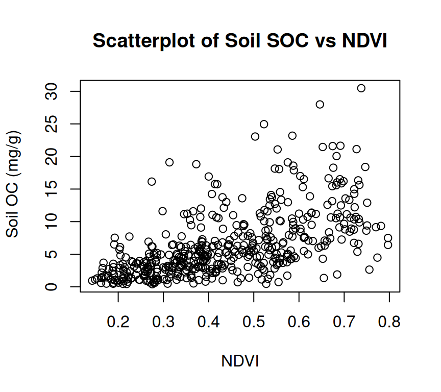
A scatter plot is a type of graph used to display the relationship between two continuous variables. This plot is commonly used in data analysis to explore and visualize the relationship between two variables. They are particularly useful in identifying patterns or trends in data, as well as in identifying outliers or unusual observations.

Code

plot(mf$NDVI, mf$SOC,
    # x-axis label 
    xlab="NDVI",
    # y-axis label
    ylab=" Soil OC (mg/g)",  
    # Plot title
    main="Scatterplot of Soil SOC vs NDVI")

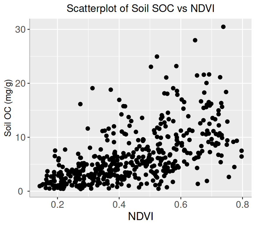
Code

ggplot(mf, aes(x=NDVI, y=SOC)) +
  geom_point(size=2) +
  # add plot title
  ggtitle("Scatterplot of Soil SOC vs NDVI") +
   theme(
    # center the plot title
    plot.title = element_text(hjust = 0.5),
    axis.line = element_line(colour = "gray"),
    # axis title font size
    axis.title.x = element_text(size = 14), 
    # X and  axis font size
    axis.text.y=element_text(size=12,vjust = 0.5, hjust=0.5),
    axis.text.x = element_text(size=12))+
     xlab("NDVI") + 
     ylab("Soil OC (mg/g)")

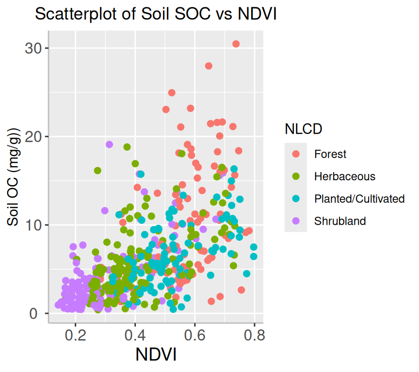
Code

ggplot(mf, aes(x=NDVI, y=SOC, color=NLCD)) +
  geom_point(size=2) +
# add plot title
  ggtitle("Scatterplot of Soil SOC vs NDVI") +
   theme(
    # center the plot title
    plot.title = element_text(hjust = 0.5),
    axis.line = element_line(colour = "gray"),
    # axis title font size
    axis.title.x = element_text(size = 14), 
    # X and  axis font size
    axis.text.y=element_text(size=12,vjust = 0.5, hjust=0.5),
    axis.text.x = element_text(size=12))+
      # add legend tittle
  guides(color = guide_legend(title = "NLCD"))+
  xlab("NDVI") + 
  ylab("Soil OC (mg/g))")

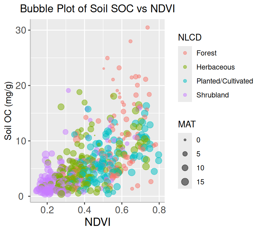
Bubble Plot

A bubble plot is a type of chart that displays data points in a 3-dimensional space using bubbles or spheres. The chart is similar to a scatter plot, but each data point is represented by a bubble with a size proportional to a third variable. Bubble plots are useful for displaying relationships between three variables and can be particularly effective when used to visualize large datasets.

Code

mf  |> 
  arrange(desc(SOC))  |> 
  mutate(NLCD = factor(NLCD))  |> 
  ggplot(aes(x=NDVI, y=SOC, size = MAT, color=NLCD)) +
    geom_point(alpha=0.5) +
    scale_size(range = c(.2, 4), name="MAT")+
     guides(color = guide_legend(title = "NLCD"))+
  ggtitle("Bubble Plot of Soil SOC vs NDVI") +
   theme(
    # center the plot title
    plot.title = element_text(hjust = 0.5),
    axis.line = element_line(colour = "gray"),
    # axis title font size
    axis.title.x = element_text(size = 14), 
    # X and  axis font size
    axis.text.y=element_text(size=12,vjust = 0.5, hjust=0.5),
    axis.text.x = element_text(size=12))+
      # add legend tittle
  guides(color = guide_legend(title = "NLCD")) + 
  xlab("NDVI") + 
  ylab("Soil OC (mg/g)")

Mariginal Plot

A marginal plot is a type of visualization that displays the distribution of a single variable along the margins of a scatterplot. It is a useful tool for exploring the relationship between two variables and can provide additional insights into the data. We will use ggMarginal() function from ggExtra library makes it create marginal plots

install.packages(“ggExtra”)

install.packages(“gridExtra”)

Code

#library(ggExtra)
# classic plot :
p<-ggplot(mf, aes(x=SOC, y=NDVI, color=NLCD, size=MAT)) +
      geom_point() +
      theme(legend.position="none") +
      xlab("NDVI") + ylab("Soil SOC (mg/g)")
p_hist <- ggMarginal(p, type="histogram", size=10)
# marginal density
p_dens <- ggMarginal(p, type="density")
# marginal boxplot
p_box <- ggMarginal(p, type="boxplot")

Code

#library(gridExtra)
grid.arrange(p_hist, p_dens, p_box, ncol=3)

Marginal Plot with Statistical Results

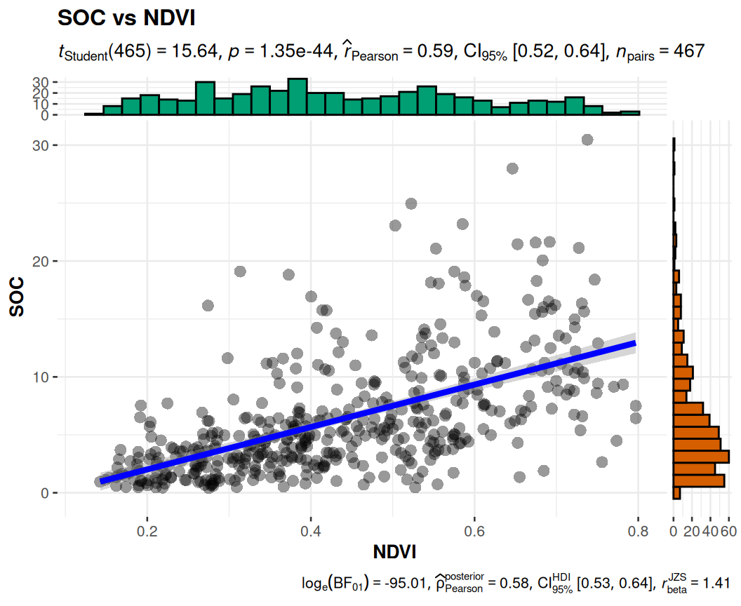
ggscatterstats() function from ggstatsplot will create scatterplots from ggplot2 combined with marginal densigram (density + histogram) plots with statistical details.

install.package(ggstatsplot)

install.package(ggside)

Code

#library(ggstatsplot )
ggstatsplot::ggscatterstats(
  data = mf, 
  x = NDVI, 
  y = SOC,
  title = "SOC vs NDVI",
  messages = FALSE
)

Correlation Matrix

A correlation matrix is a table that displays the correlation coefficients between different variables.

The rcorr() function of Hmisc package computes a matrix of Pearson’s r or Spearman’s rho rank correlation coefficients for all possible pairs of columns of a matrix.

install.packages(“Hmisc”)

Code

#library(Hmisc)
# create a data frame for correlation analysis
df.cor<-mf  |>  dplyr::select(SOC, DEM, Slope, TPI, NDVI, MAP, MAT) 
# correlation matrix
cor.mat<-Hmisc::rcorr(as.matrix(df.cor, type="pearson"))
cor.mat

        SOC   DEM Slope   TPI  NDVI   MAP   MAT
SOC    1.00  0.17  0.40  0.04  0.59  0.50 -0.36
DEM    0.17  1.00  0.70  0.00 -0.07 -0.31 -0.81
Slope  0.40  0.70  1.00 -0.01  0.31  0.15 -0.64
TPI    0.04  0.00 -0.01  1.00  0.07  0.14  0.00
NDVI   0.59 -0.07  0.31  0.07  1.00  0.80 -0.21
MAP    0.50 -0.31  0.15  0.14  0.80  1.00  0.06
MAT   -0.36 -0.81 -0.64  0.00 -0.21  0.06  1.00

n= 467 


P
      SOC    DEM    Slope  TPI    NDVI   MAP    MAT   
SOC          0.0003 0.0000 0.3745 0.0000 0.0000 0.0000
DEM   0.0003        0.0000 0.9559 0.1404 0.0000 0.0000
Slope 0.0000 0.0000        0.7940 0.0000 0.0016 0.0000
TPI   0.3745 0.9559 0.7940        0.1201 0.0017 0.9187
NDVI  0.0000 0.1404 0.0000 0.1201        0.0000 0.0000
MAP   0.0000 0.0000 0.0016 0.0017 0.0000        0.1922
MAT   0.0000 0.0000 0.0000 0.9187 0.0000 0.1922

We can create a correlation matrix table with correlation coefficients (r) and with significat P-values using following function:

Code

# install.packages("xtable")
library(xtable)

cor_table <- function(x){ 
  require(Hmisc) 
  x <- as.matrix(x) 
  R <- rcorr(x)$r 
  p <- rcorr(x)$P 
  
  ## define notions for significance levels; spacing is important.
  mystars <- ifelse(p < .001, "***", ifelse(p < .01, "** ", ifelse(p < .05, "* ", " ")))
  
  ## trunctuate the matrix that holds the correlations to three decimal
  R <- format(round(cbind(rep(-1.11, ncol(x)), R), 3))[,-1] 
  
  ## build a new matrix that includes the correlations with their apropriate stars 
  Rnew <- matrix(paste(R, mystars, sep=""), ncol=ncol(x)) 
  diag(Rnew) <- paste(diag(R), " ", sep="") 
  rownames(Rnew) <- colnames(x) 
  colnames(Rnew) <- paste(colnames(x), "", sep="") 
  
  ## remove upper triangle
  Rnew <- as.matrix(Rnew)
  Rnew[upper.tri(Rnew, diag = TRUE)] <- ""
  Rnew <- as.data.frame(Rnew) 
  
  ## remove last column and return the matrix (which is now a data frame)
  Rnew <- cbind(Rnew[1:length(Rnew)-1])
  return(Rnew) 
}

Code

cor_table(df.cor)

            SOC       DEM     Slope       TPI      NDVI     MAP
SOC                                                            
DEM    0.167***                                                
Slope  0.405***  0.703***                                      
TPI      0.041    -0.003    -0.012                             
NDVI   0.587***   -0.068   0.311***    0.072                   
MAP    0.499*** -0.308***  0.146**   0.145**   0.804***        
MAT   -0.358*** -0.808*** -0.638***    0.005  -0.210***  0.060

Pairs Plots

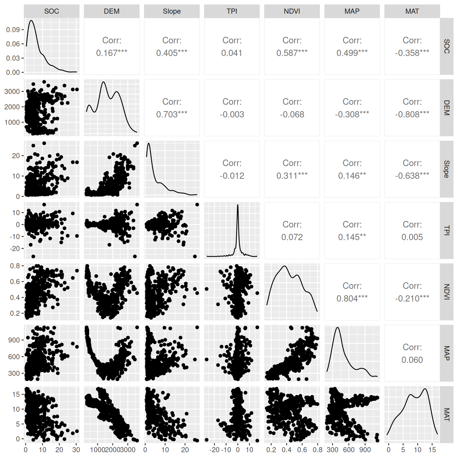
The function ggpairs() from GGally leverages a modular design of pairwise comparisons of multivariate data and displays either the density or count of the respective variable along the diagonal.

install.packages(GGally)

Code

# Load GGally library
#library(GGally)
GGally::ggpairs(df.cor)

Correlation Matrix Plots

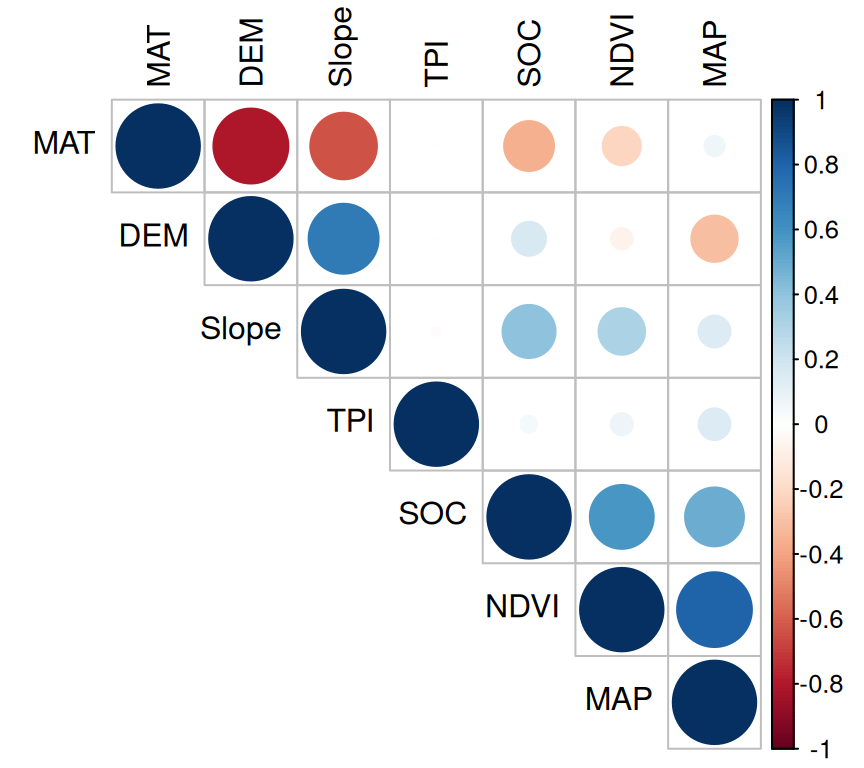
You can create a graphical display of a correlation matrix using the function corrplot() of corrplot package. The function corrplot() takes the correlation matrix as the first argument. The second argument (type=“upper”) is used to display only the upper triangular of the correlation matrix. The correlation matrix is reordered according to the correlation coefficient using “hclust” method.

install.pacakges(“corrplot”)

Code

# Load corrplot library
#library(corrplot)
# Create plot
corrplot(cor.mat$r, 
         type="upper", 
         order="hclust", 
         cex.lab = 0.5,
         tl.col = "black",
         p.mat = cor.mat$p, 
         sig.level = 0.05, insig = "blank")

In above plot, correlation coefficients are colored according to the value. Correlation matrix can be also reordered according to the degree of association between variables. Positive correlations are displayed in blue and negative correlations in red color. Color intensity and the size of the circle are proportional to the correlation coefficients. In the right side of the correlogram, the legend color shows the correlation coefficients and the corresponding colors. The correlations with p-value > 0.05 are considered as insignificant. In this case the correlation coefficient values are leaved blank.

Correlation analysis with rstatix

The ‘rstatix’ package is a user-friendly tool that follows the ‘tidyverse’ design philosophy to perform basic statistical tests, including ‘t-test’, ‘Wilcoxon test’, ‘ANOVA’, ‘Kruskal-Wallis’ and ‘correlation analyses’ with ease. The output of each test is transformed into a tidy data frame for easy visualization. Additional functions are included to help with the analysis of factorial experiments, including purely ‘within-Ss’ designs (repeated measures), purely ‘between-Ss’ designs, and mixed ‘within-and-between-Ss’ designs. The package also provides several effect size metrics, such as ‘eta squared’ for ANOVA, ‘Cohen’s d’ for t-test, and ‘Cramer’s V’ for the association between categorical variables. Additionally, the package includes helper functions to identify univariate and multivariate outliers, assess normality, and homogeneity of variance.

install.pcakges(“rstatix”)

Computing correlation:

cor_test(): correlation test between two or more variables using Pearson, Spearman or Kendall methods.

cor_mat(): compute correlation matrix with p-values. Returns a data frame containing the matrix of the correlation coefficients. The output has an attribute named pvalue which contains the matrix of the correlation test p-values.

cor_get_pval(): extract a correlation matrix p-values from an object of class cor_mat().

cor_pmat(): compute the correlation matrix, but returns only the p-values of the correlation tests.

as_cor_mat(): convert a cor_test object into a correlation matrix format.

Correlation test

cor_test() provides a pipe-friendly framework to perform correlation test between paired samples, using Pearson, Kendall or Spearman method. Wrapper around the function cor.test().

Correlation test between two variables

Code

mf |>  cor_test (SOC, NDVI)

# A tibble: 1 × 8
  var1  var2    cor statistic        p conf.low conf.high method 
  <chr> <chr> <dbl>     <dbl>    <dbl>    <dbl>     <dbl> <chr>  
1 SOC   NDVI   0.59      15.6 1.35e-44    0.524     0.644 Pearson

Correlation between the specified variable vs the remaining numeric variables

Code

mf |>  cor_test (SOC)

# A tibble: 14 × 8
   var1  var2         cor statistic        p conf.low conf.high method 
   <chr> <chr>      <dbl>     <dbl>    <dbl>    <dbl>     <dbl> <chr>  
 1 SOC   ID        -0.026    -0.563 5.74e- 1  -0.117    0.0648  Pearson
 2 SOC   FIPS      -0.087    -1.89  5.93e- 2  -0.177    0.00342 Pearson
 3 SOC   STATE_ID  -0.088    -1.90  5.86e- 2  -0.177    0.00317 Pearson
 4 SOC   Longitude  0.039     0.842 4   e- 1  -0.0519   0.129   Pearson
 5 SOC   Latitude   0.25      5.62  3.36e- 8   0.165    0.335   Pearson
 6 SOC   DEM        0.17      3.65  2.97e- 4   0.0771   0.254   Pearson
 7 SOC   Aspect     0.17      3.71  2.35e- 4   0.0799   0.256   Pearson
 8 SOC   Slope      0.4       9.55  7.68e-20   0.326    0.478   Pearson
 9 SOC   TPI        0.041     0.889 3.74e- 1  -0.0497   0.131   Pearson
10 SOC   KFactor   -0.12     -2.52  1.21e- 2  -0.205   -0.0256  Pearson
11 SOC   MAP        0.5      12.4   9.37e-31   0.427    0.564   Pearson
12 SOC   MAT       -0.36     -8.27  1.44e-15  -0.435   -0.276   Pearson
13 SOC   NDVI       0.59     15.6   1.35e-44   0.524    0.644   Pearson
14 SOC   SiltClay   0.18      3.98  8.15e- 5   0.0921   0.268   Pearson

Correaltion test by group

Code

mf  |> 
  group_by(NLCD) |> 
  cor_test(SOC, NDVI)

# A tibble: 4 × 9
  NLCD            var1  var2    cor statistic        p conf.low conf.high method
  <chr>           <chr> <chr> <dbl>     <dbl>    <dbl>    <dbl>     <dbl> <chr> 
1 Forest          SOC   NDVI   0.39      4.06 1.05e- 4    0.204     0.551 Pears…
2 Herbaceous      SOC   NDVI   0.53      7.55 4.04e-12    0.401     0.634 Pears…
3 Planted/Cultiv… SOC   NDVI   0.47      5.26 8.98e- 7    0.304     0.616 Pears…
4 Shrubland       SOC   NDVI   0.65      9.46 2.37e-16    0.532     0.737 Pears…

Correlation between one variable vs many

Code

mf %>% cor_test(
  vars = "SOC",
  vars2 = c("NDVI", "MAT", "MAP")
 )

# A tibble: 3 × 8
  var1  var2    cor statistic        p conf.low conf.high method 
  <chr> <chr> <dbl>     <dbl>    <dbl>    <dbl>     <dbl> <chr>  
1 SOC   NDVI   0.59     15.6  1.35e-44    0.524     0.644 Pearson
2 SOC   MAT   -0.36     -8.27 1.44e-15   -0.435    -0.276 Pearson
3 SOC   MAP    0.5      12.4  9.37e-31    0.427     0.564 Pearson

Correlation between two vectors of variables

Code

mf %>% cor_test(
  vars = c("SOC", "NDVI"),
  vars2 = c("MAT", "MAP")
 )

# A tibble: 4 × 8
  var1  var2    cor statistic         p conf.low conf.high method 
  <chr> <chr> <dbl>     <dbl>     <dbl>    <dbl>     <dbl> <chr>  
1 SOC   MAT   -0.36     -8.27 1.44e- 15   -0.435    -0.276 Pearson
2 SOC   MAP    0.5      12.4  9.37e- 31    0.427     0.564 Pearson
3 NDVI  MAT   -0.21     -4.63 4.66e-  6   -0.295    -0.122 Pearson
4 NDVI  MAP    0.8      29.2  4.95e-107    0.769     0.834 Pearson

Compute Correlation Matrix with P-values

cor_mat(): compute correlation matrix with p-values. Returns a data frame containing the matrix of the correlation coefficients. The output has an attribute named “pvalue”, which contains the matrix of the correlation test p-values.

cor_pmat(): compute the correlation matrix but returns only the p-values of the tests.

cor_get_pval(): extract a correlation matrix p-values from an object of class cor_mat(). P-values are not adjusted

Code

cor_mat<-mf  |>  
  dplyr::select(SOC, NDVI, MAP, MAT) |> 
  cor_mat()
cor_mat

# A tibble: 4 × 5
  rowname   SOC  NDVI   MAP   MAT
* <chr>   <dbl> <dbl> <dbl> <dbl>
1 SOC      1     0.59  0.5  -0.36
2 NDVI     0.59  1     0.8  -0.21
3 MAP      0.5   0.8   1     0.06
4 MAT     -0.36 -0.21  0.06  1

Significance levels of correlation:

Code

cor_mat  |> 
  cor_get_pval()

# A tibble: 4 × 5
  rowname      SOC      NDVI       MAP      MAT
  <chr>      <dbl>     <dbl>     <dbl>    <dbl>
1 SOC     0        1.35e- 44 9.37e- 31 1.44e-15
2 NDVI    1.35e-44 0         4.95e-107 4.66e- 6
3 MAP     9.37e-31 4.95e-107 0         1.92e- 1
4 MAT     1.44e-15 4.66e-  6 1.92e-  1 0

Visualizing correlation matrix:

cor_plot() visualize correlation matrix using base plot.

Code

cor_mat  |> 
  cor_reorder()  |> 
  pull_lower_triangle() |> 
  cor_plot(label = TRUE)

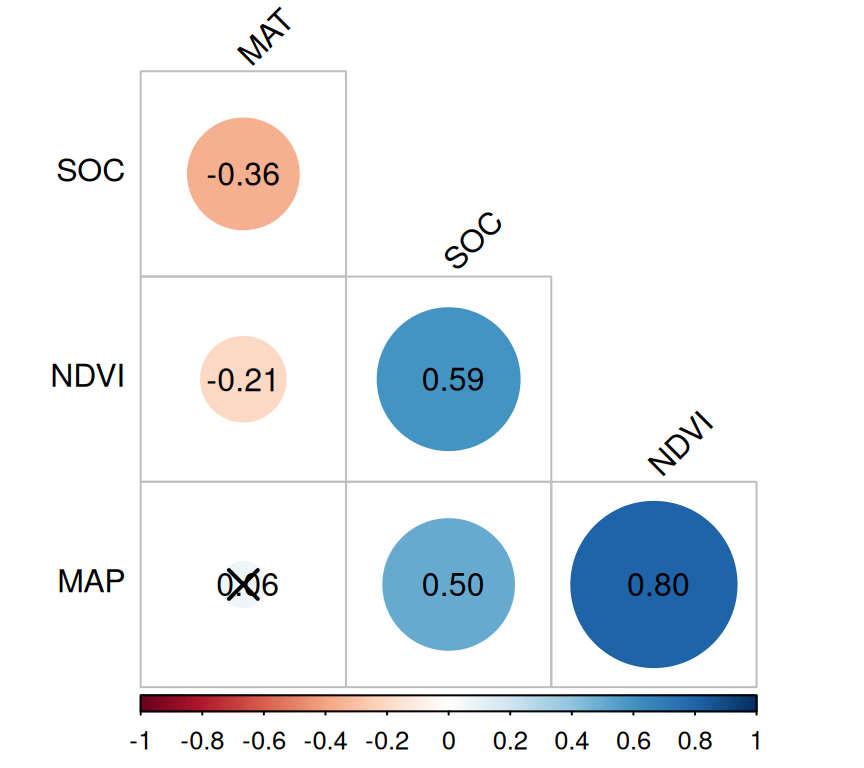
In above plot, insignificant correlations are marked by crosses.

Summary and Conclusion

The tutorial on correlation analysis in R has given you a foundation to explore relationships between variables in a dataset. You can measure the strength and direction of the relationship between two variables using correlation coefficients. With these skills, you can conduct correlation analysis on your datasets and use this foundation to explore more complex statistical techniques.

Correlation Analysis with R

Introduction

Correlation Analysis from Scratch

Correlation Analysis with R

Check and Install Required R Packages

Verify Installation

Load Packages

Check Loaded Packages

Data

Pearson Correlation

Nonparametric Correlations

Correlation Test

Correlation by Group

Scatter Plot

Bubble Plot

Mariginal Plot

Marginal Plot with Statistical Results

Correlation Matrix

Pairs Plots

Correlation Matrix Plots

Correlation analysis with rstatix

Correlation test

Correlation test between two variables

Correlation between the specified variable vs the remaining numeric variables

Correaltion test by group

Correlation between one variable vs many

Correlation between two vectors of variables

Compute Correlation Matrix with P-values

Visualizing correlation matrix:

Summary and Conclusion

References