ANOVA is widely used in various fields, including agriculture, biology, psychology, and social sciences, to analyze experimental data and draw conclusions about the effects of different treatments or factors on a response variable. Here you will learn how to perform ANOVA in R.
Introduction
Analysis of Variance (ANOVA) is a statistical technique used to compare the means of three or more groups, enabling us to determine whether there are significant differences between them. This method is widely used in research to help us understand whether the differences we observe among group means are due to genuine differences in the populations or simply random sampling variation.
ANOVA works by breaking down the total variance observed in the data into different components: the variance between group means and the variance within each group. It then examines whether the between-group variance is significantly larger than the within-group variance. If it is, this indicates that there are real differences among the groups.
There are various types of ANOVA, including one-way ANOVA, which compares the means of three or more groups on a single independent variable, and two-way ANOVA, which examines the influence of two independent variables. More complex designs, such as factorial ANOVA, can be used for multiple factors.
During ANOVA, an F-statistic is generated, which compares the ratio of the between-group variance to the within-group variance. If the calculated F-value exceeds a critical value based on the chosen significance level, usually 0.05, it suggests that there is a statistically significant difference between at least two group means.
Post-hoc tests, such as Tukey’s HSD or Bonferroni correction, are often used after ANOVA to pinpoint which specific groups differ from each other if the overall ANOVA result is significant. It’s important to note that ANOVA makes certain assumptions, such as the data following a normal distribution and the groups having equal variances. Violations of these assumptions may affect the reliability of the ANOVA results.
Overall, ANOVA is a powerful tool for comparing means across multiple groups simultaneously. It’s commonly used in various fields, such as psychology, biology, economics, and more to analyze experimental or observational data. By comparing group means, ANOVA helps us to understand the differences between groups and identify significant patterns in the data.
ANOVA tests whether the means of three or more groups are statistically different. It decomposes the total variability into:
Between-Group Variability (SSB): Differences due to group means.
Within-Group Variability (SSW): Differences due to individual observations within groups.
When conducting a research study with multiple groups, it is important to consider several factors to ensure accurate and reliable results. The first consideration is the independence of the observations. Each subject should belong to only one group, and there should be no relationship between the observations in each group. This means that having repeated measures for the same participants is not allowed, as this could introduce bias into the results.
The second consideration is the presence of any significant outliers in any design cell. Outliers are observations that fall far outside the expected range of values and can significantly impact the results of the study. Identifying and removing any outliers before analyzing the data is important to ensure accurate results.
The third consideration is normality. The data for each design cell should be approximately normally distributed, meaning that the data should follow a bell-shaped curve when plotted on a graph. Non-normal data can be transformed to meet this assumption, but this should be done carefully and with consideration of the impact on the results.
Finally, it is important to ensure homogeneity of variances. This means that the variance of the outcome variable should be equal in every design cell. If the variances are not equal, the study results could be affected, and it may be necessary to use alternative statistical methods to analyze the data.
ANOVA from scratch
Generate Synthetic Data
Code
# Set seed for reproducibilityset.seed(123)# Create synthetic data with 3 groupsgroup1 <-rnorm(10, mean =5, sd =1.5) # Group 1: mean = 5group2 <-rnorm(10, mean =6, sd =1.5) # Group 2: mean = 6group3 <-rnorm(10, mean =7, sd =1.5) # Group 3: mean = 7# Combine into a data framedata <-data.frame(weight =c(group1, group2, group3),group =factor(rep(c("Group1", "Group2", "Group3"), each =10)))# View the first few rowshead(data)
ggside: The package ggside was designed to enable users to add metadata to their ggplots with ease.
patchwork:The goal of patchwork is to make it ridiculously simple to combine separate ggplots into the same graphic.
gridExtra:The grid package provides low-level functions to create graphical objects (grobs), and position them on a page in specific viewports.
rstatix: Provides a simple and intuitive pipe-friendly framework, coherent with the ‘tidyverse’ design philosophy, for performing basic statistical tests, including t-test, Wilcoxon test, ANOVA, Kruskal-Wallis and correlation analyses.
In this exercise, we will create a data frame randomly with four treatments, six varieties, and four replications (Total 96 observation).
Code
# Set the number of observations, treatments, replications, and varietiesn <-1treatments <-4replications <-4varieties <-6# Create an empty data frame with columns for treatment, replication, variety, and observationexp.df <-data.frame(Treatment =character(),Replication =integer(),Variety =character(),Yield =numeric(),stringsAsFactors =FALSE)# Generate random data for each treatment, replication, and variety combinationfor (t in1:treatments) {for (r in1:replications) {for (v in1:varieties) {# Generate n random observations for the current combination of treatment, replication, and variety obs <-rnorm(n, mean =3*t +0.95*r +0.90*v, sd =0.25)# Add the observations to the data frame set.seeds=1256 exp.df <-rbind(exp.df, data.frame(Treatment =paste0("T", t),Replication = r,Variety =paste0("V", v),Yield = obs )) } }}# Print the first 10 rows of the data frameglimpse(exp.df)
The one-way analysis of variance (ANOVA) is used to determine whether there are any statistically significant differences between the means of two or more independent (unrelated) groups. The one-way analysis of variance (ANOVA) is a statistical test used to determine whether there are any statistically significant differences between the means of three or more independent groups.
The formula for the one-way ANOVA F-statistic is as follows:
\[ F = \frac{MSB}{MSW} \]
Where:
\(F\) is the F-statistic.
\(MSB\) is the Mean Square Between (variability between group means).
\(MSW\) is the Mean Square Within (variability within each group).
\(N\) is the total number of observations across all groups.
\(X_{ij}\) is the \(j^{th}\) observation in group \(i\).
\(\bar{X}_i\) is the mean of group \(i\).
In these formulas, \(\bar{X}_i\) represents the mean of each group, \(n_i\) is the number of observations in each group, and \(k\) is the number of groups. The F-statistic is used to assess whether the variability between group means \(MSB\) is significantly larger than the variability within each group \(MSW\), indicating whether there are significant differences between at least two group means.
The output of an ANOVA test includes an F-statistic, which is a measure of the difference between the groups, and a p-value, which indicates the probability of obtaining the observed difference by chance. If the p-value is less than a chosen significance level (typically 0.05), then the null hypothesis, which states that there is no significant difference between the means of the groups, can be rejected.
ANOVA in R can be performed using the built-in aov() function. This function takes a formula as an argument, where the dependent variable is on the left side of the tilde (~), and the independent variables are on the right side, separated by +. We will use dataset we have created before to see the main effect of treatment on yield.
Analysis of Variance Table

Response: Yield
          Df  Sum Sq Mean Sq F value    Pr(>F)
Treatment  3 1060.42  353.47  99.535 < 2.2e-16 ***
Residuals 92  326.71    3.55
---
Signif. codes:  0 '***' 0.001 '**' 0.01 '*' 0.05 '.' 0.1 ' ' 1
A nice and easy way to report results of an ANOVA in R is with the report() function from the report package
Code
report(anova.one)
The ANOVA (formula: Yield ~ Treatment) suggests that:

  - The main effect of Treatment is statistically significant and large (F(3, 92)
= 99.53, p < .001; Eta2 = 0.76, 95% CI [0.70, 1.00])

Effect sizes were labelled following Field's (2013) recommendations.
Two-way ANOVA
Two-way ANOVA (analysis of variance) or factorial ANOVA is a statistical method used to analyze the effects of two categorical independent variables, or factors, or continuous dependent variables. It tests for the main effects of each factor and their interaction effect.
In a two-way ANOVA, we consider the effects of two categorical independent variables on a continuous dependent variable. The general formula for the observed value \(Y_{ijk}\) in a two-way ANOVA is as follows:
Where: - \(Y_{ijk}\) is the observed value for the \(i^{th}\) level of the first independent variable, the \(j^{th}\) level of the second independent variable, and the \(k^{th}\) observation. - \(\mu\) is the overall mean. - \(\alpha_i\) represents the effect of the \(i^{th}\) level of the first independent variable. - \(\beta_j\) represents the effect of the \(j^{th}\) level of the second independent variable. - \((\alpha \beta)_{ij}\) is the interaction effect between the \(i^{th}\) level of the first independent variable and the \(j^{th}\) level of the second independent variable. - \(\epsilon_{ijk}\) is the random error term.
Now, let’s expand the terms for each effect:
Overall Mean (\(\mu\)):
\[ \mu = \frac{\sum_{i=1}^{a} \sum_{j=1}^{b} \sum_{k=1}^{n} Y_{ijk}}{a \cdot b \cdot n} \] Where: - \(a\) is the number of levels in the first independent variable. - \(b\) is the number of levels in the second independent variable. - \(n\) is the number of observations in each cell.
Main Effects:
Main Effect of the First Independent Variable (\(\alpha_i\)): \[ \alpha_i = \frac{\sum_{j=1}^{b} \sum_{k=1}^{n} Y_{ijk}}{b \cdot n} - \mu \]
Main Effect of the Second Independent Variable (\(\beta_j\)): \[ \beta_j = \frac{\sum_{i=1}^{a} \sum_{k=1}^{n} Y_{ijk}}{a \cdot n} - \mu \]
In these formulas, \(Y_{ijk}\) represents the observed values, \(\mu\) is the overall mean, \(\alpha_i\) and \(\beta_j\) are the main effects, \((\alpha \beta)_{ij}\)) is the interaction effect, and \(\epsilon_{ijk}\) is the random error term. These effects help explain the variability in the observed values due to the independent variables and their interaction. The goal of two-way ANOVA is to test the significance of these effects.
Here is an example code for a two-way ANOVA with one dependent variable (Yield), and two independent variables (Treatment and Variety) with interaction effect:
From the ANOVA table we can conclude that both Treatment and Variety statistically significant.
Code
report(anova.two)
The ANOVA (formula: Yield ~ Treatment + Variety + Treatment:Variety) suggests
that:

  - The main effect of Treatment is statistically significant and large (F(3, 72)
= 223.14, p < .001; Eta2 (partial) = 0.90, 95% CI [0.87, 1.00])
  - The main effect of Variety is statistically significant and large (F(5, 72) =
26.79, p < .001; Eta2 (partial) = 0.65, 95% CI [0.53, 1.00])
  - The interaction between Treatment and Variety is statistically not
significant and very small (F(15, 72) = 0.02, p > .999; Eta2 (partial) =
4.37e-03, 95% CI [0.00, 1.00])

Effect sizes were labelled following Field's (2013) recommendations.
Multiple Comparisons
After performing an ANOVA, if the overall F-test is significant, we may want to determine which groups differ significantly from each other in terms of the dependent variable. This can be done using post-hoc tests or multiple comparison tests.
When conducting a study with three or more groups and analyzing the data using ANOVA or a similar statistical test, you may encounter a significant difference among the group means. However, this result does not provide information about which specific pairs of group means differ significantly from each other. To identify these differences, you can use multiple comparison procedures.
Multiple comparisons refer to a set of statistical techniques that allow you to conduct pairwise comparisons between the means of different groups in a study. These comparisons are performed after a significant result in ANOVA or a similar test and help you identify which specific groups have significantly different means.
There are several ways to perform multiple comparisons, including pairwise t-tests, Tukey’s HSD test, Scheffe’s test and Bonferroni correction. Each procedure has its strengths and weaknesses, and the choice of which one to use depends on various factors, such as the number of groups being compared and the desired level of statistical significance.
Using multiple comparison procedures is crucial in statistical analysis as it helps you avoid making false conclusions by controlling the overall risk of making a Type I error. By identifying which specific pairs of group means are significantly different from each other, you can gain a more comprehensive understanding of your data, which can inform future research and decision-making.
Tukey’s Honestly Significant Difference (HSD) test
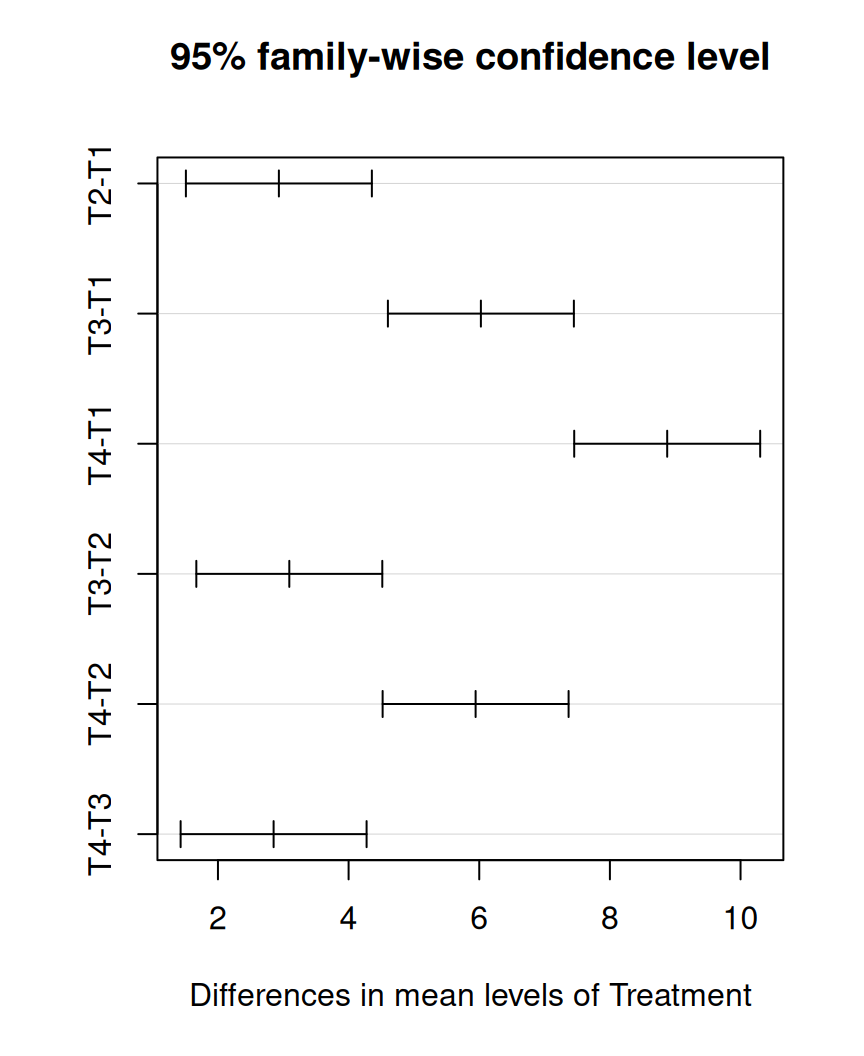
Tukey’s Honestly Significant Difference (HSD) test is a powerful statistical method that is commonly used in experimental research to compare multiple groups and determine if their means significantly differ from each other. One of the major advantages of the HSD test is that it controls the familywise error rate, which means it helps to reduce the likelihood of making a type I error (false positive) when comparing groups. This is achieved by providing a confidence interval that helps to identify which pairs of group means differ significantly from each other, while maintaining an appropriate level of statistical significance. Overall, Tukey’s HSD test is a reliable tool that can help researchers make accurate and informed decisions when analyzing experimental data.
In R, the TukeyHSD() function can be used to perform Tukey’s HSD test, which returns a table of pairwise comparisons between the groups, along with the adjusted p-values:
The table shows the differences between the groups and the 95% confidence intervals for each difference. If the confidence interval does not include zero, the difference between the groups is significant at the specified level.
Instead of printing the TukeyHSD results in a table, we’ll do it in a graph
Code
plot(tukey.one)
Pairewise t-test
The pairwise.t.test() function can be used to perform Bonferroni correction or other multiple comparison tests. For example, to perform pairwise comparisons using Bonferroni correction, we can use:
    Pairwise comparisons using t tests with pooled SD

data:  exp.df$Yield and exp.df$Treatment

   T1      T2      T3
T2 3.2e-06 -       -
T3 < 2e-16 9.2e-07 -
T4 < 2e-16 < 2e-16 6.0e-06

P value adjustment method: bonferroni
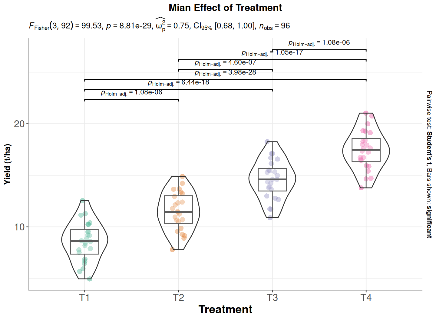
Box/Violin plots for between-subjects comparisons
We can create a nice looking plots with results of ANOVA and post-hoc tests on the same plot (directly on the boxplots). We will use gbetweenstats() function of ggstatsplot package:
install.packages(“ggstatsplot”)
Code
p1<-ggstatsplot::ggbetweenstats(data = exp.df,x = Treatment,y = Yield,ylab ="Yield (t/ha)",type ="parametric", # ANOVA or Kruskal-Wallisvar.equal =TRUE, # ANOVA or Welch ANOVAplot.type ="box",pairwise.comparisons =TRUE,pairwise.display ="significant",centrality.plotting =FALSE,bf.message =FALSE)+# add plot titleggtitle("Mian Effect of Treatment") +theme(# center the plot titleplot.title =element_text(hjust =0.5),axis.line =element_line(colour ="gray"),# axis title font sizeaxis.title.x =element_text(size =14), # X and axis font sizeaxis.text.y=element_text(size=12,vjust =0.5, hjust=0.5),axis.text.x =element_text(size=12))print(p1)
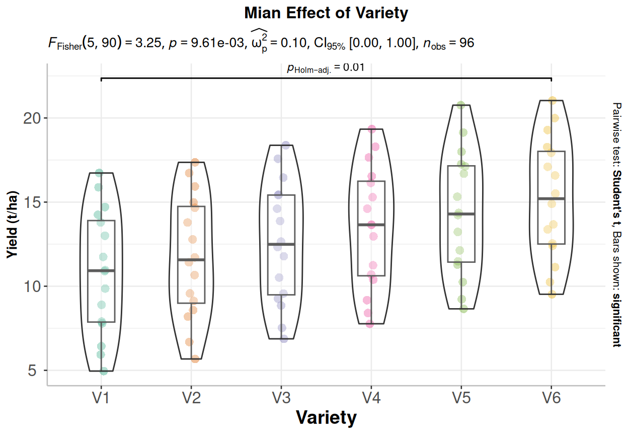
Code
# Load library#library(ggstatsplot)p2<-ggbetweenstats(data = exp.df,x = Variety,y = Yield,ylab ="Yield (t/ha)",type ="parametric", # ANOVA or Kruskal-Wallisvar.equal =TRUE, # ANOVA or Welch ANOVAplot.type ="box",pairwise.comparisons =TRUE,pairwise.display ="significant",centrality.plotting =FALSE,bf.message =FALSE)+# add plot titleggtitle("Mian Effect of Variety") +theme(# center the plot titleplot.title =element_text(hjust =0.5),axis.line =element_line(colour ="gray"),# axis title font sizeaxis.title.x =element_text(size =14), # X and axis font sizeaxis.text.y=element_text(size=12,vjust =0.5, hjust=0.5),axis.text.x =element_text(size=12))print(p2)
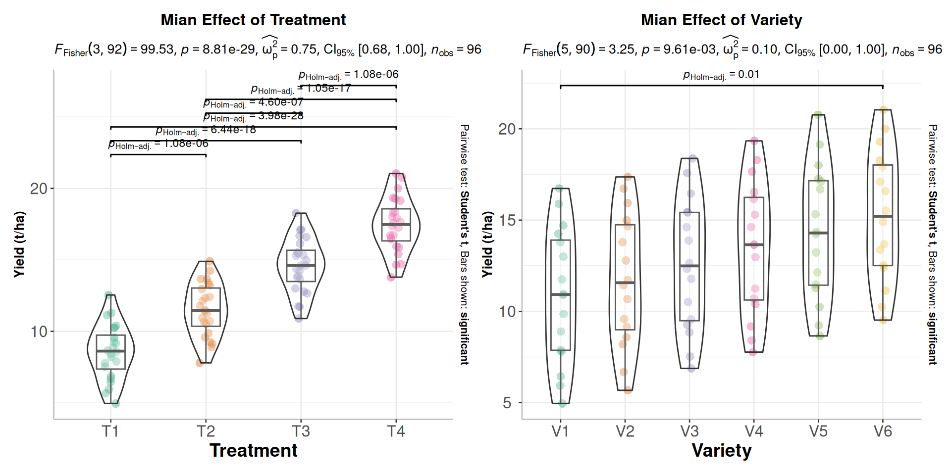
We plot these plots side by side using patchwork package:
install.packages(“patchwork”)
Code
#library(patchwork)p1+p2
ANOVA with rstatix
anova_test() function in rstatix’ package is an easy to use wrapper around Anova() and aov(). It makes ANOVA computation handy in R and It’s highly flexible: can support model and formula as input. Variables can be also specified as character vector using the arguments dv, wid, between, within, covariate.
One-way ANOVA test
Code
exp.df |>anova_test (Yield ~Treatment)
ANOVA Table (type II tests)

     Effect DFn DFd      F        p p<.05   ges
1 Treatment   3  92 99.535 8.81e-29     * 0.764
This tutorial explains how to conduct ANOVA analysis in R. ANOVA is a technique used to compare means across groups, popular in fields like business, psychology, medicine, and engineering. It helps identify differences between groups, which can inform decision-making and further research.
Remember the assumptions underlying ANOVA, including normality, homogeneity of variances, and independence. Conduct appropriate post hoc tests to determine which groups differ significantly. Consider the effect size when interpreting ANOVA results, and avoid making causal inferences. Mastering ANOVA analysis in R can help you better understand your data and make more informed decisions.