Code
packages <- c('tidyverse',
         'SmartEDA',
         'ggthemes'

)![]()

In this tutorial, we will guide you through the various features of the {SmartEDA} package for EDA. The package is particularly useful for both beginners and experienced data analysts, as it simplifies the process of EDA while still providing powerful capabilities.
The {SmartEDA} package provides a quick way to generate a summary of the dataset using the ExpData() function. This function gives an overview of the data, including basic statistics and data type information. It provides detailed summaries, visualizations, and diagnostics to analyze datasets effectively. Key features:
Auto-generated statistics (numeric and categorical variables).
Interactive visualizations (histograms, bar plots, scatterplots, etc.).
Missing value analysis and correlation matrices.
Flexible customization for variables and report structure.
Shiny app integration for dynamic exploration.
packages <- c('tidyverse',
'SmartEDA',
'ggthemes'
)#| warning: false
#| error: false
# Install missing packages
new_packages <- packages[!(packages %in% installed.packages()[,"Package"])]
if(length(new_packages)) install.packages(new_packages)
# Verify installation
cat("Installed packages:\n")
print(sapply(packages, requireNamespace, quietly = TRUE))# Load packages with suppressed messages
invisible(lapply(packages, function(pkg) {
suppressPackageStartupMessages(library(pkg, character.only = TRUE))
}))# Check loaded packages
cat("Successfully loaded packages:\n")Successfully loaded packages:print(search()[grepl("package:", search())]) [1] "package:ggthemes" "package:SmartEDA" "package:lubridate"
[4] "package:forcats" "package:stringr" "package:dplyr"
[7] "package:purrr" "package:readr" "package:tidyr"
[10] "package:tibble" "package:ggplot2" "package:tidyverse"
[13] "package:stats" "package:graphics" "package:grDevices"
[16] "package:utils" "package:datasets" "package:methods"
[19] "package:base" The data set use in this exercise can be downloaded from my Dropbox or from my Github account.
We will use read_csv() function of readr package to import data as a tidy data.
mf<-read_csv("https://github.com/zia207/r-colab/raw/main/Data/R_Beginners/gp_soil_data_na.csv")The ExpData() function is the main function provided by the SmartEDA package. It generates a summary of the dataset, including key statistics for each variable. The type argument specifies the level of summary:
type = 1: Provides basic information like data types, missing values, and unique values.type = 2: Offers a more detailed summary, including distribution statistics. mf |> dplyr::select(NLCD, SOC, DEM, MAP, MAT, NDVI) |>
SmartEDA::ExpData(type = 1) Descriptions Value
1 Sample size (nrow) 471
2 No. of variables (ncol) 6
3 No. of numeric/interger variables 5
4 No. of factor variables 0
5 No. of text variables 1
6 No. of logical variables 0
7 No. of identifier variables 0
8 No. of date variables 0
9 No. of zero variance variables (uniform) 0
10 %. of variables having complete cases 83.33% (5)
11 %. of variables having >0% and <50% missing cases 16.67% (1)
12 %. of variables having >=50% and <90% missing cases 0% (0)
13 %. of variables having >=90% missing cases 0% (0)# detail summary
mf |> dplyr::select(NLCD, SOC, DEM, MAP, MAT, NDVI) |>
SmartEDA::ExpData(type = 2) Index Variable_Name Variable_Type Sample_n Missing_Count Per_of_Missing
1 1 NLCD character 471 0 0.000
2 2 SOC numeric 467 4 0.008
3 3 DEM numeric 471 0 0.000
4 4 MAP numeric 471 0 0.000
5 5 MAT numeric 471 0 0.000
6 6 NDVI numeric 471 0 0.000
No_of_distinct_values
1 4
2 456
3 464
4 464
5 463
6 464To compute detailed descriptive statistics for numeric and categorical variables, you can use the ExpnsNumStat() and ExpCatStat() functions.
Key arguments:
by: Specifies whether to compute statistics for all variables or by group.Qnt: Quantiles to calculate.Outlier: If TRUE, identifies outliers.# Summary statistics for numeric variables
mf |> dplyr::select(NLCD, SOC, DEM, MAP, MAT, NDVI) |>
SmartEDA::ExpNumStat() Vname Group TN nNeg nZero nPos NegInf PosInf NA_Value Per_of_Missing
2 DEM All 471 0 0 471 0 0 0 0.000
3 MAP All 471 0 0 471 0 0 0 0.000
4 MAT All 471 6 0 465 0 0 0 0.000
5 NDVI All 471 0 0 471 0 0 0 0.000
1 SOC All 471 0 0 467 0 0 4 0.849
sum min max mean median SD CV IQR Skewness
2 768251.070 258.649 3618.024 1631.106 1592.893 767.692 0.471 1058.934 -0.023
3 235204.661 193.913 1128.115 499.373 432.630 206.936 0.414 237.652 1.079
4 4185.080 -0.591 16.874 8.886 9.173 4.098 0.461 6.564 -0.274
5 205.088 0.142 0.797 0.435 0.416 0.162 0.372 0.251 0.233
1 2965.806 0.408 30.473 6.351 4.971 5.045 0.794 5.944 1.460
Kurtosis
2 -0.808
3 0.452
4 -0.828
5 -0.921
1 2.388Stat - summary statistics, IV - information value
df <- mf |>
  dplyr::select(NLCD, SOC, DEM, MAP, MAT, NDVI)

ExpCatStat(df,
           Target="NLCD",
           result = "Stat",
           clim=10,
           nlim=10,bins=10,
           Pclass=1,
           plot=FALSE,
           top=20,
           Round=2)
Warning in FUN(X[[i]], ...): NAs introduced by coercion Variable Target Unique Chi-squared p-value df IV Value Cramers V
1 SOC NLCD 9 42.543 0.003 NA 0 0.19
2 DEM NLCD 10 515.564 0.000 NA 0 0.60
3 MAP NLCD 10 280.146 0.000 NA 0 0.45
4 MAT NLCD 10 346.840 0.000 NA 0 0.50
5 NDVI NLCD 10 344.735 0.000 NA 0 0.49
Degree of Association Predictive Power
1 Moderate Not Predictive
2 Strong Not Predictive
3 Strong Not Predictive
4 Strong Not Predictive
5 Strong Not Predictive# Information value plot
ExpCatStat(df,
Target="NLCD",
result = "Stat",
clim=10,
nlim=10,bins=10,
Pclass=1,
plot=TRUE,
top=20,
Round=2)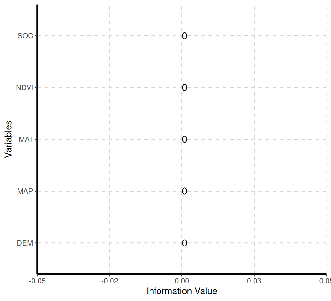
  Variable Target Unique Chi-squared p-value df IV Value Cramers V
1      SOC   NLCD      9      42.543   0.001 NA        0      0.19
2      DEM   NLCD     10     515.564   0.000 NA        0      0.60
3      MAP   NLCD     10     280.146   0.000 NA        0      0.45
4      MAT   NLCD     10     346.840   0.000 NA        0      0.50
5     NDVI   NLCD     10     344.735   0.000 NA        0      0.49
  Degree of Association Predictive Power
1              Moderate   Not Predictive
2                Strong   Not Predictive
3                Strong   Not Predictive
4                Strong   Not Predictive
5                Strong   Not Predictive
Information value (IV) is a measure of the predictive power of a categorical variable in relation to a target variable (Weight of evidence and Information values). It quantifies how well a categorical variable can differentiate between different classes or outcomes in the target variable. The IV is calculated based on the distribution of the categorical variable across different classes of the target variable.
Criteria used for categorical variable predictive power classification are
IV is < 0.03then predictive power =Not Predictive
IV is 0.3 to 0.1 then predictive power = Somewhat Predictive
IV 0.1 to 0.3 then predictive power = Meidum Predictive
>0.3 then predictive power = Highly Predictive
ExpCatStat(df,
           Target="NLCD",
           result = "IV",
           clim=10,
           nlim=10,bins=10,
           Pclass=1,
           plot=TRUE,
           top=20,
           Round=2)
Variable Class Out_1 Out_0 TOTAL Per_1 Per_0 Odds WOE IV Ref_1
1 SOC.1 [1.286,2.304] 47 47 94 0.10 0.10 1 0 0 1
2 SOC.2 (2.304,3.105] 47 47 94 0.10 0.10 1 0 0 1
3 SOC.3 (3.105,3.983] 47 47 94 0.10 0.10 1 0 0 1
4 SOC.4 (3.983,4.971] 47 47 94 0.10 0.10 1 0 0 1
5 SOC.5 (4.971,6.123] 46 46 92 0.10 0.10 1 0 0 1
6 SOC.6 (6.123,7.5] 47 47 94 0.10 0.10 1 0 0 1
7 SOC.7 (7.5,10.076] 48 48 96 0.10 0.10 1 0 0 1
8 SOC.8 (10.076,13.351] 45 45 90 0.10 0.10 1 0 0 1
9 SOC.9 <NA> 97 97 194 0.21 0.21 1 0 0 1
10 DEM.1 [258.649,439.696] 47 47 94 0.10 0.10 1 0 0 1
11 DEM.2 (439.696,924.605] 47 47 94 0.10 0.10 1 0 0 1
12 DEM.3 (924.605,1261.5] 47 47 94 0.10 0.10 1 0 0 1
13 DEM.4 (1261.5,1395.63] 47 47 94 0.10 0.10 1 0 0 1
14 DEM.5 (1395.63,1592.89] 48 48 96 0.10 0.10 1 0 0 1
15 DEM.6 (1592.89,1876.87] 47 47 94 0.10 0.10 1 0 0 1
16 DEM.7 (1876.87,2164.8] 47 47 94 0.10 0.10 1 0 0 1
17 DEM.8 (2164.8,2334.02] 47 47 94 0.10 0.10 1 0 0 1
18 DEM.9 (2334.02,2620.15] 47 47 94 0.10 0.10 1 0 0 1
19 DEM.10 (2620.15,3618.02] 47 47 94 0.10 0.10 1 0 0 1
20 MAP.1 [193.913,290.205] 47 47 94 0.10 0.10 1 0 0 1
21 MAP.2 (290.205,340.257] 47 47 94 0.10 0.10 1 0 0 1
22 MAP.3 (340.257,369.653] 47 47 94 0.10 0.10 1 0 0 1
23 MAP.4 (369.653,403.034] 47 47 94 0.10 0.10 1 0 0 1
24 MAP.5 (403.034,432.63] 48 48 96 0.10 0.10 1 0 0 1
25 MAP.6 (432.63,471.39] 47 47 94 0.10 0.10 1 0 0 1
26 MAP.7 (471.39,557.498] 47 47 94 0.10 0.10 1 0 0 1
27 MAP.8 (557.498,663.027] 47 47 94 0.10 0.10 1 0 0 1
28 MAP.9 (663.027,835.669] 47 47 94 0.10 0.10 1 0 0 1
29 MAP.10 (835.669,1128.11] 47 47 94 0.10 0.10 1 0 0 1
30 MAT.1 [-0.591064,2.81879] 47 47 94 0.10 0.10 1 0 0 1
31 MAT.2 (2.81879,5.00161] 47 47 94 0.10 0.10 1 0 0 1
32 MAT.3 (5.00161,6.81505] 47 47 94 0.10 0.10 1 0 0 1
33 MAT.4 (6.81505,7.5714] 47 47 94 0.10 0.10 1 0 0 1
34 MAT.5 (7.5714,9.17284] 48 48 96 0.10 0.10 1 0 0 1
35 MAT.6 (9.17284,10.5666] 47 47 94 0.10 0.10 1 0 0 1
36 MAT.7 (10.5666,11.8026] 47 47 94 0.10 0.10 1 0 0 1
37 MAT.8 (11.8026,12.7932] 47 47 94 0.10 0.10 1 0 0 1
38 MAT.9 (12.7932,13.9399] 47 47 94 0.10 0.10 1 0 0 1
39 MAT.10 (13.9399,16.8743] 47 47 94 0.10 0.10 1 0 0 1
40 NDVI.1 [0.142433,0.21877] 47 47 94 0.10 0.10 1 0 0 1
41 NDVI.2 (0.21877,0.275361] 47 47 94 0.10 0.10 1 0 0 1
42 NDVI.3 (0.275361,0.330886] 47 47 94 0.10 0.10 1 0 0 1
43 NDVI.4 (0.330886,0.376435] 47 47 94 0.10 0.10 1 0 0 1
44 NDVI.5 (0.376435,0.415683] 48 48 96 0.10 0.10 1 0 0 1
45 NDVI.6 (0.415683,0.477347] 47 47 94 0.10 0.10 1 0 0 1
46 NDVI.7 (0.477347,0.534857] 47 47 94 0.10 0.10 1 0 0 1
47 NDVI.8 (0.534857,0.585367] 47 47 94 0.10 0.10 1 0 0 1
48 NDVI.9 (0.585367,0.675952] 47 47 94 0.10 0.10 1 0 0 1
49 NDVI.10 (0.675952,0.796992] 47 47 94 0.10 0.10 1 0 0 1
Ref_0 Target
1 Shrubland, Forest, Planted/Cultivated, Herbaceous NLCD
2 Shrubland, Forest, Planted/Cultivated, Herbaceous NLCD
3 Shrubland, Forest, Planted/Cultivated, Herbaceous NLCD
4 Shrubland, Forest, Planted/Cultivated, Herbaceous NLCD
5 Shrubland, Forest, Planted/Cultivated, Herbaceous NLCD
6 Shrubland, Forest, Planted/Cultivated, Herbaceous NLCD
7 Shrubland, Forest, Planted/Cultivated, Herbaceous NLCD
8 Shrubland, Forest, Planted/Cultivated, Herbaceous NLCD
9 Shrubland, Forest, Planted/Cultivated, Herbaceous NLCD
10 Shrubland, Forest, Planted/Cultivated, Herbaceous NLCD
11 Shrubland, Forest, Planted/Cultivated, Herbaceous NLCD
12 Shrubland, Forest, Planted/Cultivated, Herbaceous NLCD
13 Shrubland, Forest, Planted/Cultivated, Herbaceous NLCD
14 Shrubland, Forest, Planted/Cultivated, Herbaceous NLCD
15 Shrubland, Forest, Planted/Cultivated, Herbaceous NLCD
16 Shrubland, Forest, Planted/Cultivated, Herbaceous NLCD
17 Shrubland, Forest, Planted/Cultivated, Herbaceous NLCD
18 Shrubland, Forest, Planted/Cultivated, Herbaceous NLCD
19 Shrubland, Forest, Planted/Cultivated, Herbaceous NLCD
20 Shrubland, Forest, Planted/Cultivated, Herbaceous NLCD
21 Shrubland, Forest, Planted/Cultivated, Herbaceous NLCD
22 Shrubland, Forest, Planted/Cultivated, Herbaceous NLCD
23 Shrubland, Forest, Planted/Cultivated, Herbaceous NLCD
24 Shrubland, Forest, Planted/Cultivated, Herbaceous NLCD
25 Shrubland, Forest, Planted/Cultivated, Herbaceous NLCD
26 Shrubland, Forest, Planted/Cultivated, Herbaceous NLCD
27 Shrubland, Forest, Planted/Cultivated, Herbaceous NLCD
28 Shrubland, Forest, Planted/Cultivated, Herbaceous NLCD
29 Shrubland, Forest, Planted/Cultivated, Herbaceous NLCD
30 Shrubland, Forest, Planted/Cultivated, Herbaceous NLCD
31 Shrubland, Forest, Planted/Cultivated, Herbaceous NLCD
32 Shrubland, Forest, Planted/Cultivated, Herbaceous NLCD
33 Shrubland, Forest, Planted/Cultivated, Herbaceous NLCD
34 Shrubland, Forest, Planted/Cultivated, Herbaceous NLCD
35 Shrubland, Forest, Planted/Cultivated, Herbaceous NLCD
36 Shrubland, Forest, Planted/Cultivated, Herbaceous NLCD
37 Shrubland, Forest, Planted/Cultivated, Herbaceous NLCD
38 Shrubland, Forest, Planted/Cultivated, Herbaceous NLCD
39 Shrubland, Forest, Planted/Cultivated, Herbaceous NLCD
40 Shrubland, Forest, Planted/Cultivated, Herbaceous NLCD
41 Shrubland, Forest, Planted/Cultivated, Herbaceous NLCD
42 Shrubland, Forest, Planted/Cultivated, Herbaceous NLCD
43 Shrubland, Forest, Planted/Cultivated, Herbaceous NLCD
44 Shrubland, Forest, Planted/Cultivated, Herbaceous NLCD
45 Shrubland, Forest, Planted/Cultivated, Herbaceous NLCD
46 Shrubland, Forest, Planted/Cultivated, Herbaceous NLCD
47 Shrubland, Forest, Planted/Cultivated, Herbaceous NLCD
48 Shrubland, Forest, Planted/Cultivated, Herbaceous NLCD
49 Shrubland, Forest, Planted/Cultivated, Herbaceous NLCDExpCustomStat{} fuction You can customize the summary statistics. Output returns matrix object containing descriptive information on all input variables for each level or combination of levels in categorical/group variable. Also while running the analysis user can filter out the data by individual variable level or across data level.
ExpCustomStat(df,
               Cvar="NLCD",                 # categorical variable to group by
             Nvar = c("SOC","NDVI"),        # quantitative variables on which to run summary statistics for.
             stat = c("Count","sum","var", "mean"), #  descriptive statistics
             gpby = TRUE)                   # group by categorical variable
NLCD Attribute Count sum var mean
<char> <char> <int> <num> <num> <num>
1: Shrubland SOC 130 524.60700 14.02396956 4.1307638
2: Forest SOC 93 970.07200 46.26920463 10.4308817
3: Planted/Cultivated SOC 97 649.58200 12.94777281 6.6967216
4: Herbaceous SOC 151 821.54500 15.40634178 5.4769667
5: Shrubland NDVI 130 39.85538 0.01678473 0.3065798
6: Forest NDVI 93 53.06253 0.01334062 0.5705648
7: Planted/Cultivated NDVI 97 51.72287 0.01471496 0.5332255
8: Herbaceous NDVI 151 60.44728 0.01708390 0.4003131ExpStat() provides bivariate summary statistics for all the categorical predictors against target variables. Output includes chi - square value, degrees of freedom, information value, p-value
X = Independent categorical variable.
Y = Binary response variable, it can take values of either 1 or 0.
The function provides summary statistics like
Unique number of levels
Chi square statistics
P value
df Degrees of freedom
IV Information value
Predictive class
data("mtcars")
X = mtcars$carb
Y = mtcars$am
ExpStat(X,Y,valueOfGood = 1)
X-squared
[1,] "6"
[2,] "6.237"
[3,] "0.264"
[4,] NA
[5,] "0.17"
[6,] "0.44"
[7,] "Strong"
[8,] "Somewhat Predictive"The {SmartEDA} package includes several visualization tools for data exploration. The ExpNumViz() function is particularly useful for creating visual summaries.
# Visualize data distributions
ExpNumViz(df, nlim = 2,
          col = NULL,
           Page = NULL,
          sample = 4,
          scatter = FALSE,
          gtitle = "Density plot: ")
[[1]]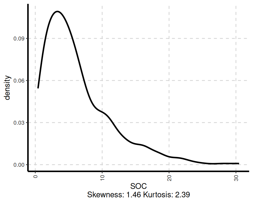
[[2]]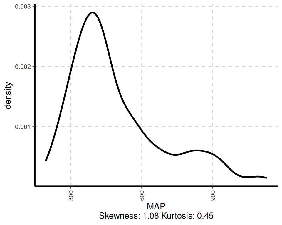
[[3]]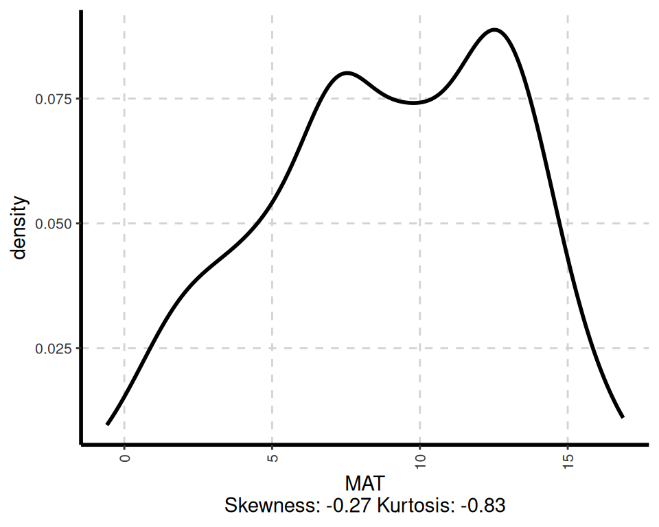
[[4]]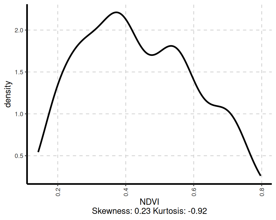
ExpNumViz(df,
          target = "NLCD", type = 2, nlim = 2,
           col = c("red", "green", "blue", "pink"),
          Page = NULL,
          sample = 4,
          scatter = FALSE,
           gtitle = "Box plot: ")
[[1]]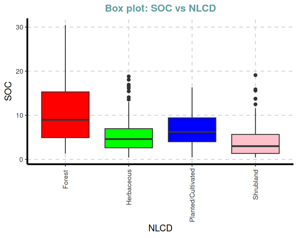
[[2]]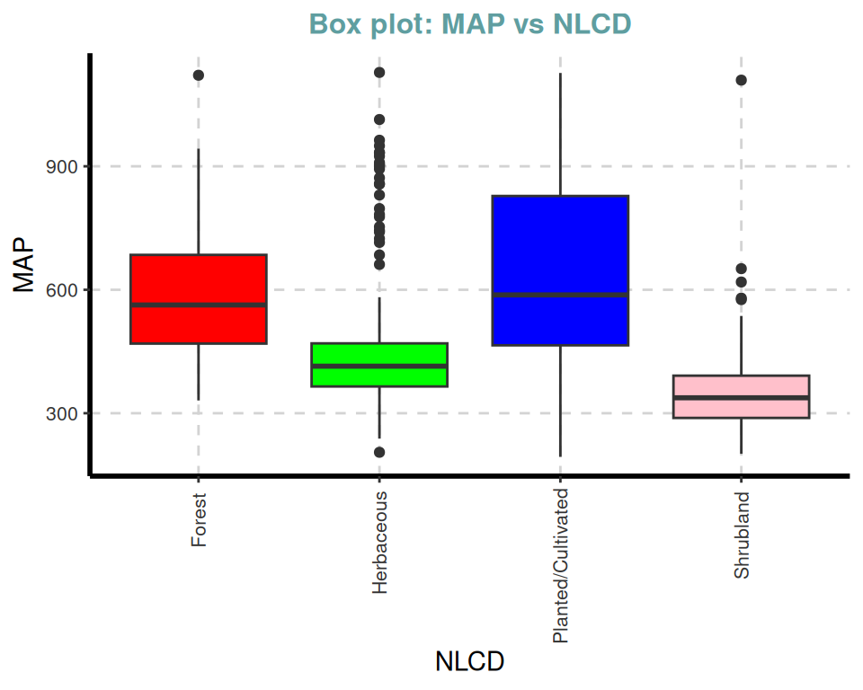
[[3]]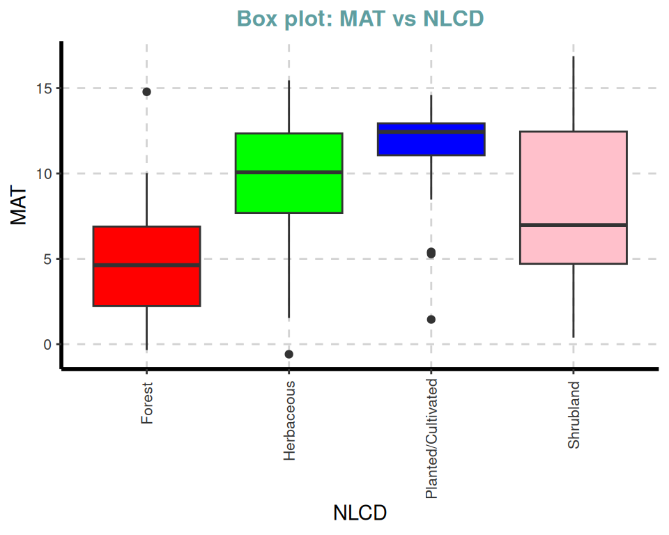
[[4]]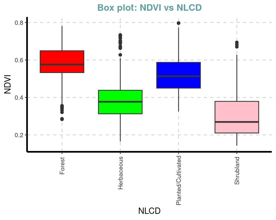
ExpNumViz(df,
          target = "SOC",
          type = 1,
          nlim = 2,
          col = "gray",
          Page = NULL, sample = NULL,
          scatter = FALSE,
          gtitle = "Scatter plot: ", theme = "Default")
[[1]]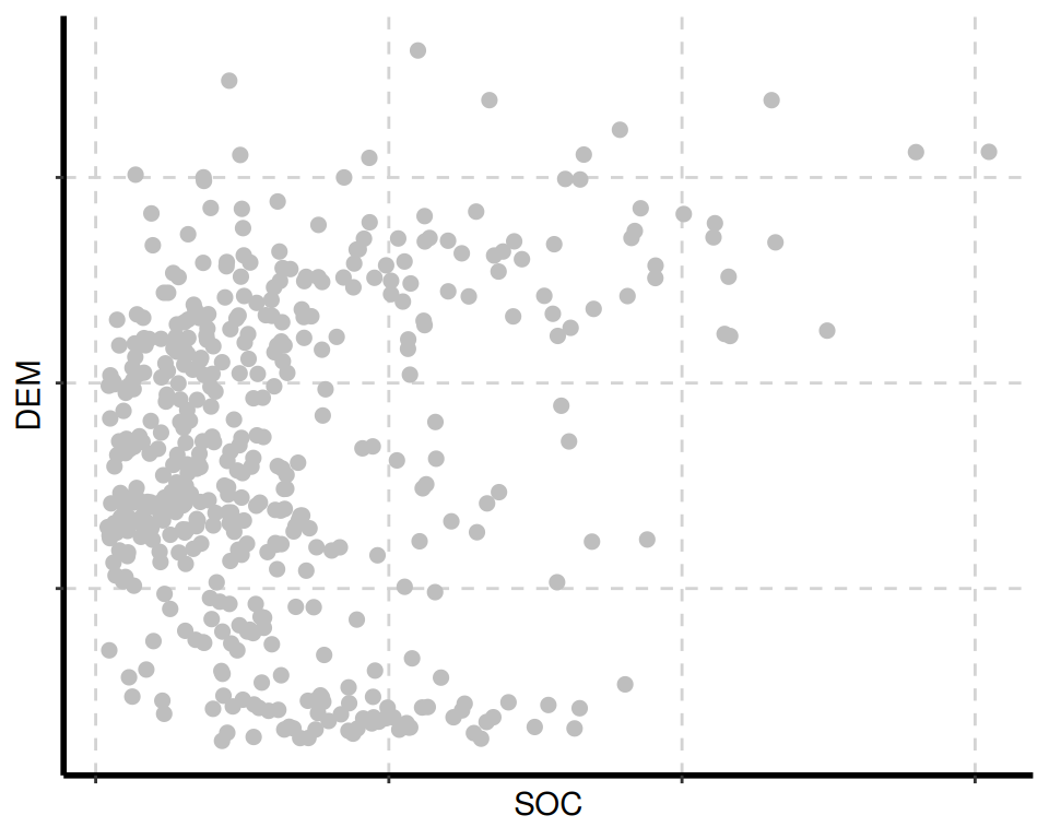
[[2]]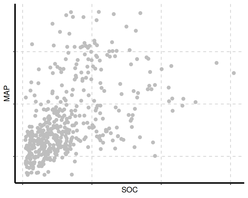
[[3]]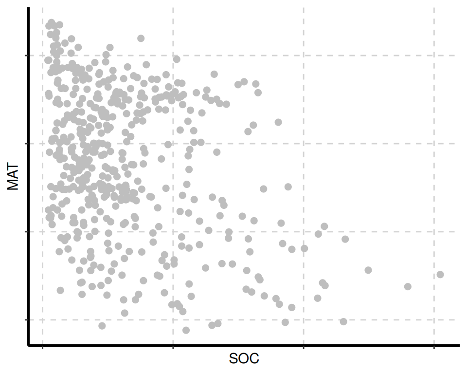
[[4]]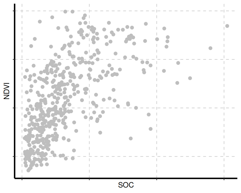
## Generate Scatter plot for all the numerical variables
ExpNumViz(df,
          target = "NLCD",
          type = 1, nlim = 2,
           col = c("red", "green", "blue"),
          Page = NULL, sample = NULL, scatter = TRUE,
           gtitle = "Scatter plot: ", theme = "Default")
[[1]]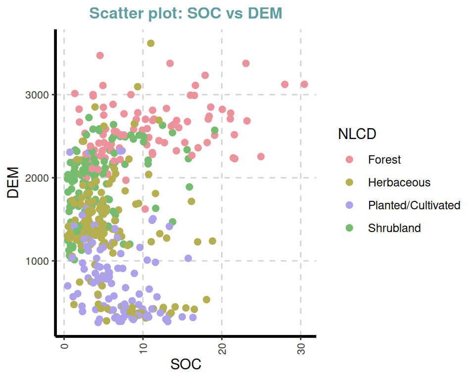
[[2]]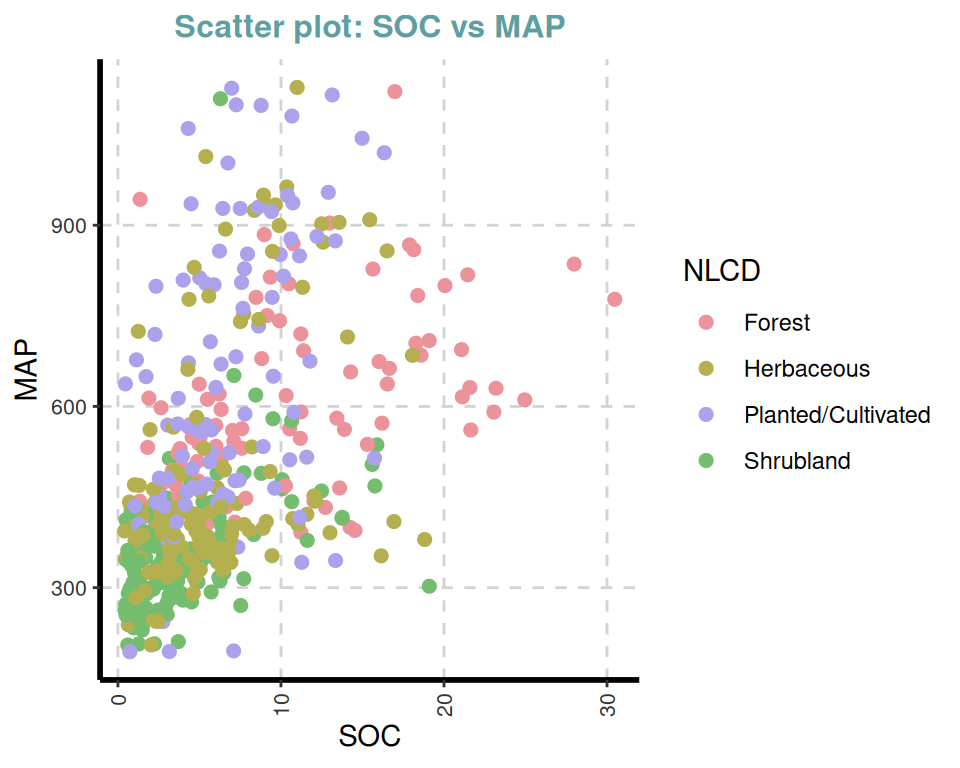
[[3]]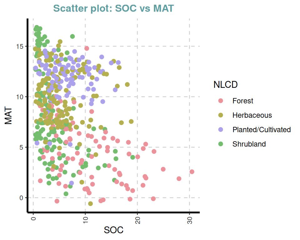
[[4]]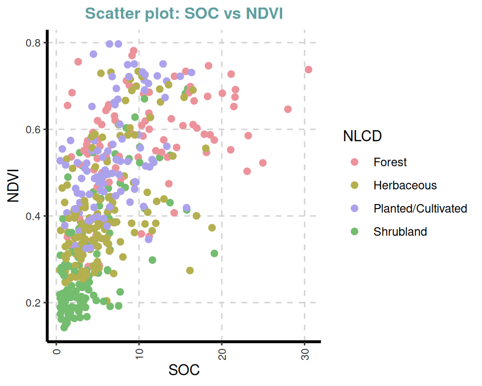
[[5]]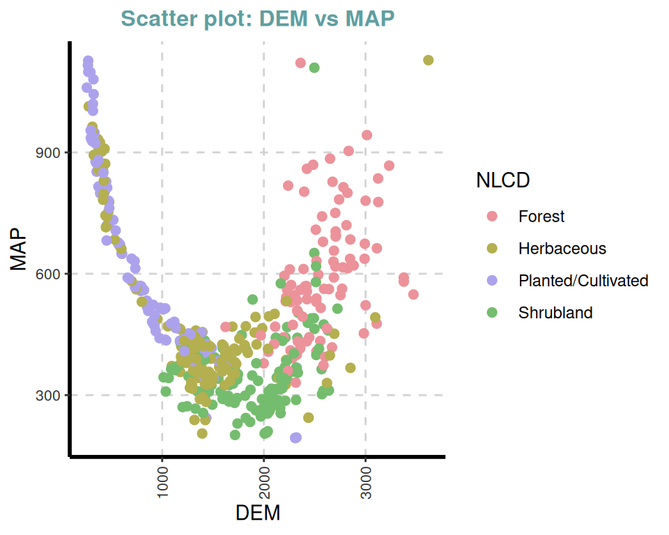
[[6]]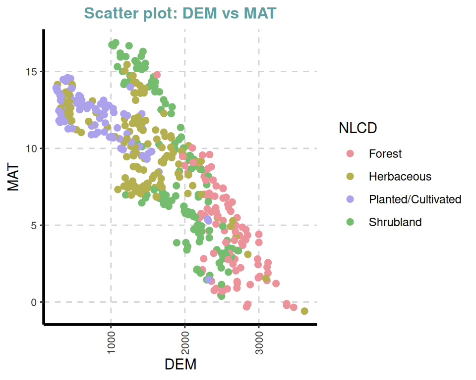
[[7]]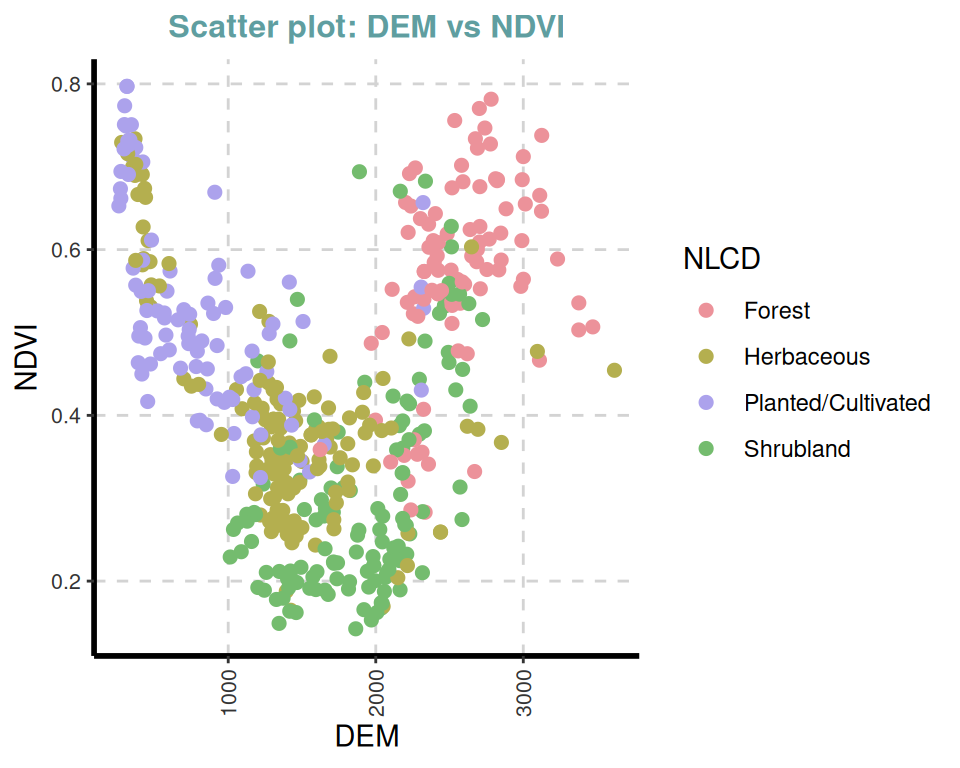
[[8]]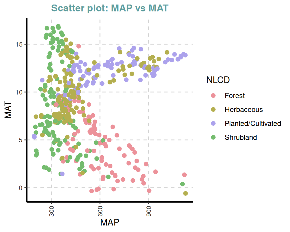
[[9]]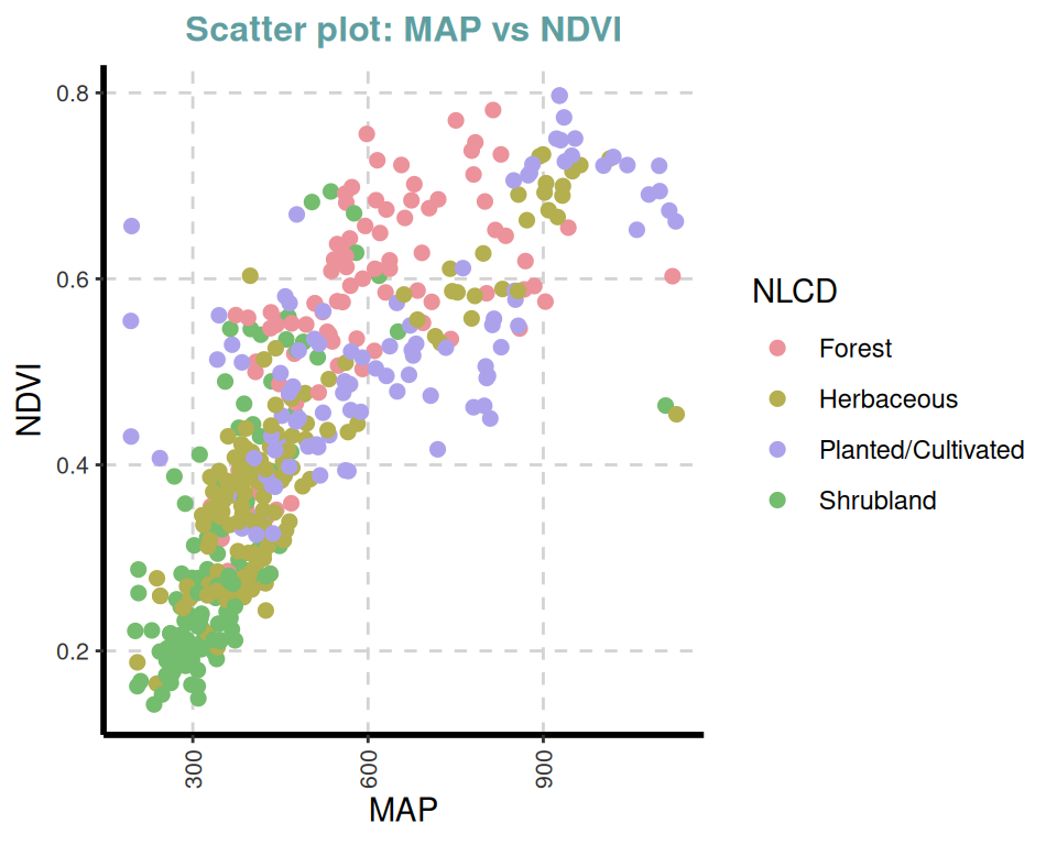
[[10]]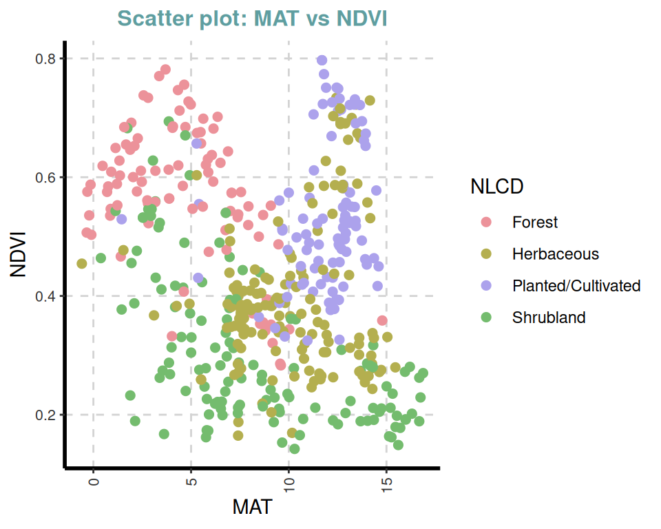
The ExpOutQQ() function generates quantile-quantile (QQ) plots to assess the normality of the data. QQ plots compare the quantiles of the data against the quantiles of a theoretical normal distribution. If the points in the QQ plot follow a straight line, it suggests that the data is normally distributed.
ExpOutQQ(df, nlim=10, fname=NULL,Page=c(2,2),sample=4)$`0`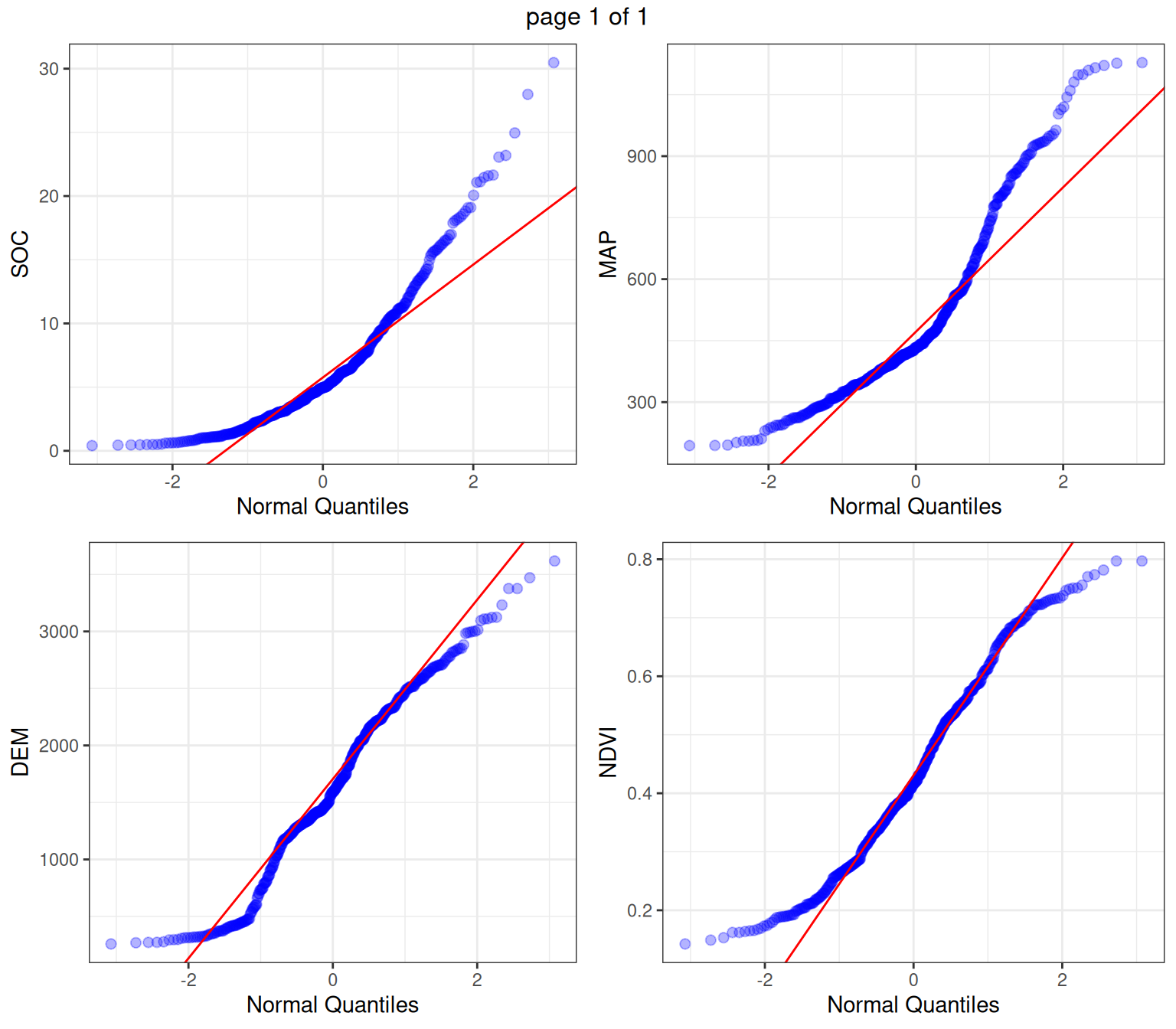
The ExpReport() function generates an HTML report summarizing the EDA results. This report includes visualizations, summary statistics, and other relevant information about the dataset.
library (ggthemes)
ExpReport(df,Target=NULL,
          label="car",theme=theme_foundation(),
op_file="Samp.html")The {SmartEDA} package is a comprehensive tool for data exploration in R. Its combination of descriptive statistics, visualization tools, and automated reporting makes it an excellent choice for both beginners and advanced users. With SmartEDA, you can streamline your EDA process and focus more on interpreting the results and deriving insights.