Functional Programming with {purrr)

The {purrr} package, part of the {tidyverse}, enhances functional programming in R by providing a consistent and user-friendly set of tools for working with functions and vectors. It builds on the concepts of functional programming, making it easier to apply functions to data structures in a more readable and efficient way.

This tutorial introduces functional programming in R using the {purrr} package. Functional programming emphasizes writing reusable, modular code by applying functions to data structures, reducing reliance on loops. purrr offers tools to make this process clean and efficient. Functional programming avoids side effects, promotes pure functions, and simplifies code. In R, {purrr} replaces loops with functions like map(), making code more readable and less error-prone.

Check and Install Required Packages

Code

packages <- c('tidyverse', 
              'broom',
              'corrplot',
             'patchwork'
              )

#| warning: false
#| error: false

# Install missing packages
new_packages <- packages[!(packages %in% installed.packages()[,"Package"])]
if(length(new_packages)) install.packages(new_packages)

Verify Installation

Code

# Verify installation
cat("Installed packages:\n")

Installed packages:

Code

print(sapply(packages, requireNamespace, quietly = TRUE))

tidyverse     broom  corrplot patchwork 
     TRUE      TRUE      TRUE      TRUE

Load Packages

Code

# Load packages with suppressed messages
invisible(lapply(packages, function(pkg) {
  suppressPackageStartupMessages(library(pkg, character.only = TRUE))
}))

Check Loaded Packages

Code

# Check loaded packages
cat("Successfully loaded packages:\n")

Successfully loaded packages:

Code

print(search()[grepl("package:", search())])

 [1] "package:patchwork" "package:corrplot"  "package:broom"    
 [4] "package:lubridate" "package:forcats"   "package:stringr"  
 [7] "package:dplyr"     "package:purrr"     "package:readr"    
[10] "package:tidyr"     "package:tibble"    "package:ggplot2"  
[13] "package:tidyverse" "package:stats"     "package:graphics" 
[16] "package:grDevices" "package:utils"     "package:datasets" 
[19] "package:methods"   "package:base"

Key purrr Functions

The `map()` Family

The map() functions apply a function to each element of a list or vector and return a list or specific output type.

map(): Returns a list.
map_dbl(), map_chr(), map_lgl(): Return vectors of type double, character, or logical.
map_df(): Returns a data frame.

Example: Squaring Numbers:

Code

numbers <- c(1, 2, 3, 4)
purrr::map_dbl(numbers, ~ .x^2)

[1]  1  4  9 16

Here, ~ .x^2 is a formula-style anonymous function where .x represents each element.

Example: Applying a Custom Function

Code

double <- function(x) x * 2
purrr::map(numbers, double)

[[1]]
[1] 2

[[2]]
[1] 4

[[3]]
[1] 6

[[4]]
[1] 8

Working with Lists

purrr excels with lists, common in R for handling complex data.

Example: Extracting Elements from a List

Code

data <- list(
  list(name = "Alice", age = 25),
  list(name = "Bob", age = 30)
)
purrr::map_chr(data, "name")

[1] "Alice" "Bob"

Iterating Over Multiple Inputs

map2() and pmap() allow functions to take multiple arguments.

Example: map2()

Code

x <- c(1, 2, 3)
y <- c(10, 20, 30)
purrr::map2_dbl(x, y, ~ .x + .y)

[1] 11 22 33

Example: pmap()

Code

params <- list(
  x = c(1, 2, 3),
  y = c(10, 20, 30),
  z = c(100, 200, 300)
)
purrr::pmap_dbl(params, ~ ..1 + ..2 + ..3)

[1] 111 222 333

Here, ..1, ..2, ..3 refer to the first, second, and third arguments.

Conditional Mapping

keep(): Retain elements where a condition is TRUE.
discard(): Remove elements where a condition is TRUE.

Example: Filtering Numbers

Code

numbers <- c(1, 2, 3, 4, 5)
purrr::keep(numbers, ~ .x > 3)

[1] 4 5

Code

purrr::discard(numbers, ~ .x > 3)

[1] 1 2 3

Reducing Lists

reduce() combines elements of a list into a single result.

Example: Summing a List

Code

map(numbers, ~ .x * 10)  |>  reduce(`+`) # Returns: 150

[1] 150

The |> pipe passes the result of map() to reduce().

Data Frame Manipulation

Suppose you have a data frame and want to calculate summary statistics for numeric columns.

Code

df <- tibble(
  a = c(1, 2, 3),
  b = c(4, 5, 6),
  c = c("x", "y", "z")
)

# Apply mean() to numeric columns
df |> 
  select(where(is.numeric))  |> 
  map_dbl(mean)

a b 
2 5

Best Practices

Use formula syntax (~) for simple anonymous functions.
Choose the appropriate map_*() function for the desired output type.
Combine with tidyverse pipes for readable workflows.
Avoid side effects (e.g., modifying global variables) to keep functions pure.

Functional Programming with {purr}r: A Real-World Example

In this section, we will demonstrate functional programming using the purrr package to process a dataset containing Age Adjusted Lung & Bronchus Cancer Mortality Rates along with various covariates from 1998 to 2010. The goal is to split the dataset by year and write each subset to a separate CSV file and performs descriptive statistics, correlation analysis, and creates correlation matrix plots for each year.

Data

Age-adjusted lung and bronchus cancer mortality rates (1998–2010) by county were obtained from IHME and estimated using spatial Bayesian mixed effects models (Mokdad et al., 2016), incorporating seven sociodemographic covariates. To address small-sample instability, rates were smoothed using an Empirical Bayesian smoother in SpaceStat.

Age-standardized cigarette smoking prevalence by county (1996–2012) was estimated from BRFSS data using logistic hierarchical mixed effects models by sex, with age standardization to the 2000 census (Dwyer-Lindgren et al., 2014). Uncertainty was assessed via simulation.

County-level poverty rates came from the U.S. Census SAIPE program, combining survey data, population estimates, and administrative records.

PM2.5, NO2, and SO2 annual concentrations (1998–2012) were derived from satellite data (e.g., MODIS, GOME) and models, validated with ground measurements. All pollutant rasters were resampled to 2.5 km × 2 km using Empirical Bayesian Kriging (ArcGIS) and population-weighted means were calculated per county.

Code

data<-read_csv("https://raw.githubusercontent.com/zia207/Data/main/CSV_files/data_1998_2010_long_lbc.csv")

Rows: 46605 Columns: 10
── Column specification ────────────────────────────────────────────────────────
Delimiter: ","
dbl (10): FIPS, X, Y, Year, SMOKING, POVERTY, PM25, NO2, SO2, RATE

ℹ Use `spec()` to retrieve the full column specification for this data.
ℹ Specify the column types or set `show_col_types = FALSE` to quiet this message.

Split Data by Year and Write to CSV Files

The code avoids loops by leveraging purrr::walk(), which is designed for side effects like writing files. Each output file contains all columns from the original dataset for the corresponding year.

Get Unique Years: Extracts unique years from the Year column using unique().
Iterate with walk(): The walk() function iterates over each year, filters the data for that year, creates a filename (e.g., data_1998.csv), and writes the subset to a CSV file using write.csv(). The message() function provides feedback on each file written.

Code

# Verify data
stopifnot("Year" %in% names(data))
cat("Data dimensions:", dim(data), "\n")

Data dimensions: 46605 10

Code

print(head(data$Year))

[1] 1998 1999 2000 2001 2002 2003

Code

# Set working directory (ensure it exists!)
dir_path <- "/home/zia207/R_Websites/R_Beginner"
if (!dir.exists(dir_path)) dir.create(dir_path, recursive = TRUE)
setwd(dir_path)

Code

# Write yearly files
unique_years <- unique(data$Year)
walk(unique_years, ~ {
  year_data <- data %>% filter(Year == .x)
  filename <- paste0("data_", .x, ".csv")
  write_csv(year_data, filename)  # use write_csv from readr for consistency
  message("Written: ", filename, " (rows: ", nrow(year_data), ")")
})

Code

# Now read them back
files <- list.files(pattern = "^data_\\d{4}\\.csv$", full.names = TRUE)
years <- str_extract(basename(files), "\\d{4}")

if (length(files) == 0) {
  stop("No CSV files found! Check working directory and file writing.")
}

select_numeric_cols <- function(df) {
  df %>% select(SMOKING, POVERTY, PM25, NO2, SO2, RATE)
}

data_list <- map(files, ~ read_csv(.x) %>% select_numeric_cols()) %>% 
  set_names(years)

Rows: 3107 Columns: 10
── Column specification ────────────────────────────────────────────────────────
Delimiter: ","
dbl (10): FIPS, X, Y, Year, SMOKING, POVERTY, PM25, NO2, SO2, RATE

ℹ Use `spec()` to retrieve the full column specification for this data.
ℹ Specify the column types or set `show_col_types = FALSE` to quiet this message.
Rows: 3107 Columns: 10
── Column specification ────────────────────────────────────────────────────────
Delimiter: ","
dbl (10): FIPS, X, Y, Year, SMOKING, POVERTY, PM25, NO2, SO2, RATE

ℹ Use `spec()` to retrieve the full column specification for this data.
ℹ Specify the column types or set `show_col_types = FALSE` to quiet this message.
Rows: 3107 Columns: 10
── Column specification ────────────────────────────────────────────────────────
Delimiter: ","
dbl (10): FIPS, X, Y, Year, SMOKING, POVERTY, PM25, NO2, SO2, RATE

ℹ Use `spec()` to retrieve the full column specification for this data.
ℹ Specify the column types or set `show_col_types = FALSE` to quiet this message.
Rows: 3107 Columns: 10
── Column specification ────────────────────────────────────────────────────────
Delimiter: ","
dbl (10): FIPS, X, Y, Year, SMOKING, POVERTY, PM25, NO2, SO2, RATE

ℹ Use `spec()` to retrieve the full column specification for this data.
ℹ Specify the column types or set `show_col_types = FALSE` to quiet this message.
Rows: 3107 Columns: 10
── Column specification ────────────────────────────────────────────────────────
Delimiter: ","
dbl (10): FIPS, X, Y, Year, SMOKING, POVERTY, PM25, NO2, SO2, RATE

ℹ Use `spec()` to retrieve the full column specification for this data.
ℹ Specify the column types or set `show_col_types = FALSE` to quiet this message.
Rows: 3107 Columns: 10
── Column specification ────────────────────────────────────────────────────────
Delimiter: ","
dbl (10): FIPS, X, Y, Year, SMOKING, POVERTY, PM25, NO2, SO2, RATE

ℹ Use `spec()` to retrieve the full column specification for this data.
ℹ Specify the column types or set `show_col_types = FALSE` to quiet this message.
Rows: 3107 Columns: 10
── Column specification ────────────────────────────────────────────────────────
Delimiter: ","
dbl (10): FIPS, X, Y, Year, SMOKING, POVERTY, PM25, NO2, SO2, RATE

ℹ Use `spec()` to retrieve the full column specification for this data.
ℹ Specify the column types or set `show_col_types = FALSE` to quiet this message.
Rows: 3107 Columns: 10
── Column specification ────────────────────────────────────────────────────────
Delimiter: ","
dbl (10): FIPS, X, Y, Year, SMOKING, POVERTY, PM25, NO2, SO2, RATE

ℹ Use `spec()` to retrieve the full column specification for this data.
ℹ Specify the column types or set `show_col_types = FALSE` to quiet this message.
Rows: 3107 Columns: 10
── Column specification ────────────────────────────────────────────────────────
Delimiter: ","
dbl (10): FIPS, X, Y, Year, SMOKING, POVERTY, PM25, NO2, SO2, RATE

ℹ Use `spec()` to retrieve the full column specification for this data.
ℹ Specify the column types or set `show_col_types = FALSE` to quiet this message.
Rows: 3107 Columns: 10
── Column specification ────────────────────────────────────────────────────────
Delimiter: ","
dbl (10): FIPS, X, Y, Year, SMOKING, POVERTY, PM25, NO2, SO2, RATE

ℹ Use `spec()` to retrieve the full column specification for this data.
ℹ Specify the column types or set `show_col_types = FALSE` to quiet this message.
Rows: 3107 Columns: 10
── Column specification ────────────────────────────────────────────────────────
Delimiter: ","
dbl (10): FIPS, X, Y, Year, SMOKING, POVERTY, PM25, NO2, SO2, RATE

ℹ Use `spec()` to retrieve the full column specification for this data.
ℹ Specify the column types or set `show_col_types = FALSE` to quiet this message.
Rows: 3107 Columns: 10
── Column specification ────────────────────────────────────────────────────────
Delimiter: ","
dbl (10): FIPS, X, Y, Year, SMOKING, POVERTY, PM25, NO2, SO2, RATE

ℹ Use `spec()` to retrieve the full column specification for this data.
ℹ Specify the column types or set `show_col_types = FALSE` to quiet this message.
Rows: 3107 Columns: 10
── Column specification ────────────────────────────────────────────────────────
Delimiter: ","
dbl (10): FIPS, X, Y, Year, SMOKING, POVERTY, PM25, NO2, SO2, RATE

ℹ Use `spec()` to retrieve the full column specification for this data.
ℹ Specify the column types or set `show_col_types = FALSE` to quiet this message.
Rows: 3107 Columns: 10
── Column specification ────────────────────────────────────────────────────────
Delimiter: ","
dbl (10): FIPS, X, Y, Year, SMOKING, POVERTY, PM25, NO2, SO2, RATE

ℹ Use `spec()` to retrieve the full column specification for this data.
ℹ Specify the column types or set `show_col_types = FALSE` to quiet this message.
Rows: 3107 Columns: 10
── Column specification ────────────────────────────────────────────────────────
Delimiter: ","
dbl (10): FIPS, X, Y, Year, SMOKING, POVERTY, PM25, NO2, SO2, RATE

ℹ Use `spec()` to retrieve the full column specification for this data.
ℹ Specify the column types or set `show_col_types = FALSE` to quiet this message.

Code

cat("Loaded", length(data_list), "CSV files for years:", paste(years, collapse = ", "), "\n")

Loaded 15 CSV files for years: 1998, 1999, 2000, 2001, 2002, 2003, 2004, 2005, 2006, 2007, 2008, 2009, 2010, 2011, 2012

Descriptive Statistics

Code

# Function to compute descriptive statistics (Min, Max, Mean, 95% CI)
compute_descriptive_stats <- function(df, year) {
  desc_stats <- df %>%
    summarise(across(.cols = everything(),
                     list(
                       Min = ~min(.x, na.rm = TRUE),
                       Max = ~max(.x, na.rm = TRUE),
                       Mean = ~mean(.x, na.rm = TRUE),
                       CI_lower = ~mean(.x, na.rm = TRUE) - qt(0.975, df = sum(!is.na(.x)) - 1) * sd(.x, na.rm = TRUE) / sqrt(sum(!is.na(.x))),
                       CI_upper = ~mean(.x, na.rm = TRUE) + qt(0.975, df = sum(!is.na(.x)) - 1) * sd(.x, na.rm = TRUE) / sqrt(sum(!is.na(.x)))
                     ),
                     .names = "{.col}.{.fn}")) %>%  # Use . instead of _ to avoid multiple underscores
    pivot_longer(cols = everything(),
                 names_to = c("Variable", "Statistic"),
                 names_sep = "\\.",  # Split on .
                 values_to = "Value") %>%
    pivot_wider(names_from = Statistic,
                values_from = Value,
                values_fn = mean) %>%  # Handle any duplicates by taking mean
    mutate(Year = year) %>%
    select(Year, Variable, Min, Max, Mean, CI_lower, CI_upper)
  
  # Debug: Check for duplicates
  duplicates <- desc_stats %>%
    summarise(n = n(), .by = c(Year, Variable)) %>%
    filter(n > 1)
  if (nrow(duplicates) > 0) {
    message("Duplicates found for Year ", year, ":\n")
    print(duplicates)
  }
  
  return(desc_stats)
}

# Compute descriptive statistics for each year
desc_stats_table <- imap_dfr(data_list, ~ {
  year <- .y
  df <- .x
  compute_descriptive_stats(df, year)
})

# Round numeric columns for display
desc_stats_table <- desc_stats_table %>%
  mutate(across(where(is.numeric), ~ round(.x, 3)))

# Print the table
cat("\nDescriptive Statistics Table (Min, Max, Mean, 95% CI):\n")


Descriptive Statistics Table (Min, Max, Mean, 95% CI):

Code

print(desc_stats_table)

# A tibble: 90 × 7
   Year  Variable   Min     Max   Mean CI_lower CI_upper
   <chr> <chr>    <dbl>   <dbl>  <dbl>    <dbl>    <dbl>
 1 1998  SMOKING  11.8   37.1   26.6     26.5     26.8  
 2 1998  POVERTY   1.8   43.8   14.7     14.5     14.9  
 3 1998  PM25      1.38  26.0   12.8     12.6     13.0  
 4 1998  NO2       0.13  21.4    2.04     1.98     2.10 
 5 1998  SO2       0      0.632  0.059    0.056    0.062
 6 1998  RATE     17.4  211.    68.8     68.3     69.4  
 7 1999  SMOKING  11.3   38.2   26.8     26.6     26.9  
 8 1999  POVERTY   1.9   44.9   13.5     13.3     13.7  
 9 1999  PM25      1.71  22.8   10.8     10.6     10.9  
10 1999  NO2       0.11  16.7    2.05     1.99     2.11 
# ℹ 80 more rows

Correlation Analysis

Code

# Function to compute correlation of RATE vs other variables (r and p-value)
compute_correlations <- function(df, year) {
  variables <- c("SMOKING", "POVERTY", "PM25", "NO2", "SO2")
  cor_results <- map_dfr(variables, ~ {
    test <- cor.test(df$RATE, df[[.x]], use = "complete.obs")
    tibble(
      Variable = .x,
      r = test$estimate,
      p_value = test$p.value
    )
  }) %>%
    mutate(Year = year) %>%
    select(Year, Variable, r, p_value)
  
  return(cor_results)
}

# Compute correlations for each year
cor_table <- imap_dfr(data_list, ~ {
  year <- .y
  df <- .x
  compute_correlations(df, year)
})

# Round numeric columns for display
cor_table <- cor_table %>%
  mutate(across(where(is.numeric), ~ round(.x, 3)))

# Print the table
cat("\nCorrelation Table (RATE vs Predictors):\n")


Correlation Table (RATE vs Predictors):

Code

print(cor_table)

# A tibble: 75 × 4
   Year  Variable     r p_value
   <chr> <chr>    <dbl>   <dbl>
 1 1998  SMOKING  0.711       0
 2 1998  POVERTY  0.325       0
 3 1998  PM25     0.512       0
 4 1998  NO2      0.204       0
 5 1998  SO2      0.327       0
 6 1999  SMOKING  0.719       0
 7 1999  POVERTY  0.353       0
 8 1999  PM25     0.517       0
 9 1999  NO2      0.185       0
10 1999  SO2      0.331       0
# ℹ 65 more rows

Correlation Matrix Plot

Code

# Function to select numeric columns
select_numeric_cols <- function(df) {
  df %>% select(SMOKING, POVERTY, PM25, NO2, SO2, RATE)
}

# Function to compute correlation matrix
compute_correlation <- function(df) {
  cor_matrix <- cor(df, use = "complete.obs")
  return(cor_matrix)
}

# Function to create a correlation matrix plot as a ggplot object
create_correlation_plot <- function(cor_matrix, year) {
  # Convert correlation matrix to long format for ggplot
  cor_data <- as.data.frame(as.table(cor_matrix)) %>%
    rename(Var1 = Var1, Var2 = Var2, value = Freq) %>%
    mutate(
      Var1 = factor(Var1, levels = rownames(cor_matrix)),
      Var2 = factor(Var2, levels = colnames(cor_matrix))
    )
  
  # Create ggplot-based correlation plot
  p <- ggplot(cor_data, aes(x = Var1, y = Var2, fill = value)) +
    geom_tile(color = "white") +
    geom_text(aes(label = round(value, 2)), color = "black", size = 3) +
    scale_fill_gradient2(low = "#0571b0", high = "#ca0020", mid = "white", 
                         midpoint = 0, limit = c(-1, 1), name = "Correlation") +
    theme_minimal() +
    theme(
      axis.text.x = element_text(angle = 45, vjust = 1, hjust = 1, size = 7),
      axis.text.y = element_text(size = 7),
      axis.title = element_blank(),
      plot.title = element_text(hjust = 0.5, size = 10),
      legend.text = element_text(size = 6),
      legend.title = element_text(size = 7)
    ) +
    ggtitle(paste("Correlation Matrix -", year))
  
  return(p)
}

# List all yearly CSV files
files <- list.files(pattern = "^data_\\d{4}\\.csv$", full.names = TRUE)

# Extract years from filenames
years <- str_extract(files, "\\d{4}")

# Read all files into a named list and select numeric columns
data_list <- map(files, ~ read.csv(.x) %>% select_numeric_cols()) %>% 
  set_names(years)

# Create correlation matrix plots for each year
plot_list <- imap(data_list, ~ {
  year <- .y
  df <- .x
  
  # Compute correlation matrix
  cor_matrix <- compute_correlation(df)
  
  # Create correlation plot
  create_correlation_plot(cor_matrix, year)
}) %>% set_names(years)

# Combine all plots into a single panel with 5 rows and 3 columns
combined_plot <- wrap_plots(plot_list, nrow = 5, ncol = 3) +
  plot_annotation(
    title = "Correlation Matrices by Year",
    theme = theme(plot.title = element_text(hjust = 0.5, size = 12))
  )

# Display the combined plot
print(combined_plot)

Warning: annotation$theme is not a valid theme.
Please use `theme()` to construct themes.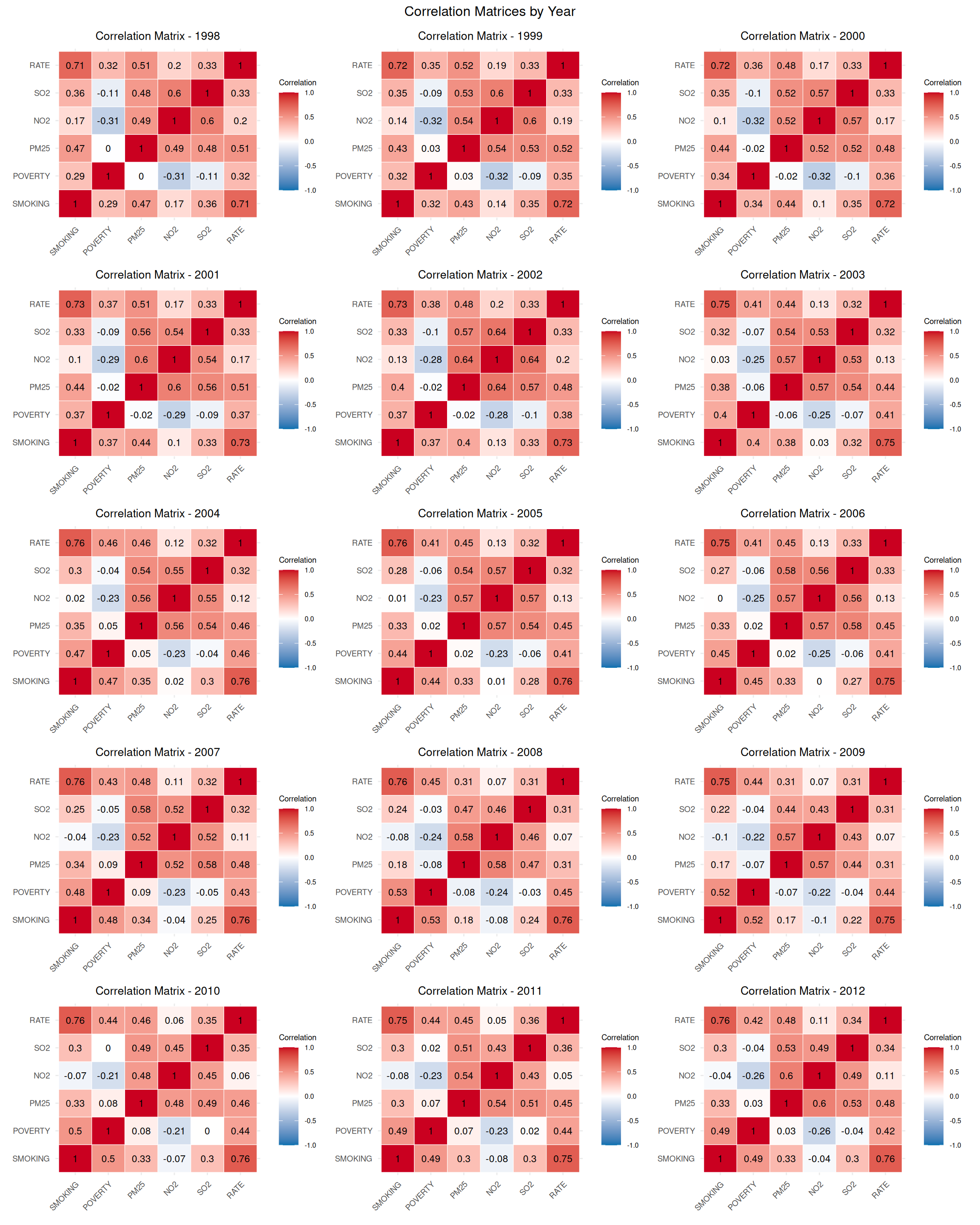

Scatter Plots

Code

# Function to select numeric columns
select_numeric_cols <- function(df) {
  df %>% select(SMOKING, RATE)
}

# Function to create scatter plot for SMOKING vs RATE
create_scatter_plot <- function(df, year) {
  p <- ggplot(df, aes(x = SMOKING, y = RATE)) +
    geom_point(color = "#1f77b4", alpha = 0.6) +
    theme_minimal() +
    labs(
      title = paste("SMOKING vs RATE -", year),
      x = "SMOKING",
      y = "RATE"
    ) +
    theme(
      plot.title = element_text(hjust = 0.5, size = 10),
      axis.title = element_text(size = 8),
      axis.text = element_text(size = 7)
    )
  
  return(p)
}

# List all yearly CSV files
files <- list.files(pattern = "^data_\\d{4}\\.csv$", full.names = TRUE)

# Extract years from filenames
years <- str_extract(files, "\\d{4}")

# Read all files into a named list using purrr::map
data_list <- map(files, read.csv) %>% set_names(years)

# Create scatter plots for each year
plot_list <- imap(data_list, ~ {
  year <- .y
  df <- .x
  
  # Select SMOKING and RATE columns
  numeric_df <- select_numeric_cols(df)
  
  # Create scatter plot
  create_scatter_plot(numeric_df, year)
}) %>% set_names(years)

# Combine all plots into a single panel with 5 rows and 3 columns
combined_plot <- wrap_plots(plot_list, nrow = 5, ncol = 3) +
  plot_annotation(
    title = "Scatter Plots of SMOKING vs RATE by Year",
    theme = theme(plot.title = element_text(hjust = 0.5))
  )

# Display the combined plot
print(combined_plot)

Warning: annotation$theme is not a valid theme.
Please use `theme()` to construct themes.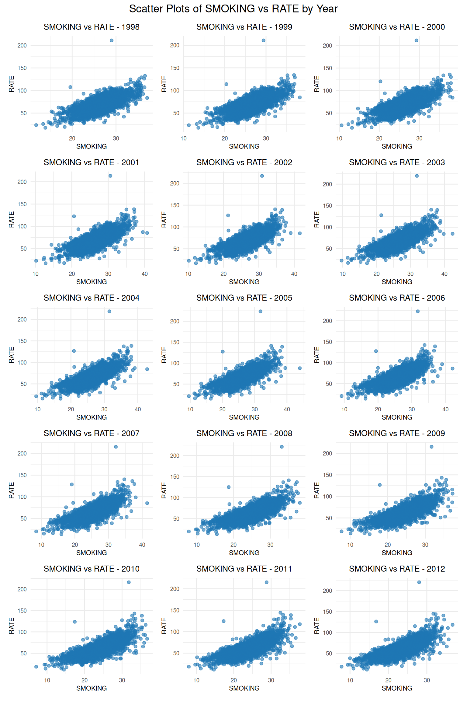

Multiple Linear Regression Analysis

Code

# Function to select numeric columns
select_numeric_cols <- function(df) {
  df %>% select(SMOKING, POVERTY, PM25, NO2, SO2, RATE)
}


# Function to fit multiple linear regression
fit_linear_regression <- function(df, year) {
  # Fit the model: RATE ~ SMOKING + POVERTY + PM25 + NO2 + SO2
  model <- lm(RATE ~ SMOKING + POVERTY + PM25 + NO2 + SO2, data = df)
  
  # Extract coefficients and R-squared using broom
  coefs <- tidy(model) %>%
    select(term, estimate) %>%
    pivot_wider(names_from = term, values_from = estimate)
  
  r_squared <- glance(model) %>%
    select(r.squared)
  
  # Combine coefficients and R-squared, add year
  result <- bind_cols(year = year, coefs, r_squared)
  
  return(result)
}

# List all yearly CSV files
files <- list.files(pattern = "^data_\\d{4}\\.csv$", full.names = TRUE)

# Extract years from filenames
years <- str_extract(files, "\\d{4}")

# Read all files into a named list using purrr::map
data_list <- map(files, read.csv) %>% set_names(years)

# Fit regression for each year and collect results
results <- imap_dfr(data_list, ~ {
  year <- .y
  df <- .x
  
  # Select numeric columns
  numeric_df <- select_numeric_cols(df)
  
  # Fit regression and get coefficients and R-squared
  fit_linear_regression(numeric_df, year)
})

# Format the table for display
results_table <- results %>%
  mutate(across(where(is.numeric), ~ round(.x, 3))) %>%
  rename(Year = year, Intercept = `(Intercept)`, R_squared = r.squared)

# Print the table
print(results_table)

# A tibble: 15 × 8
   Year  Intercept SMOKING POVERTY  PM25    NO2    SO2 R_squared
   <chr>     <dbl>   <dbl>   <dbl> <dbl>  <dbl>  <dbl>     <dbl>
 1 1998      -14.2    2.45   0.501 0.721  0.477  2.88      0.572
 2 1999      -17.1    2.49   0.515 1.15   0.128  0.739     0.596
 3 2000      -17.4    2.52   0.547 0.949  0.534  3.71      0.584
 4 2001      -17.6    2.49   0.475 1.22  -0.025  2.82      0.606
 5 2002      -19.0    2.52   0.534 1.06   0.256  3.69      0.601
 6 2003      -17.8    2.43   0.674 0.981  0.253  7.37      0.617
 7 2004      -18.5    2.43   0.554 1.26   0.095  6.03      0.636
 8 2005      -18.7    2.52   0.362 1.28   0.229  5.28      0.634
 9 2006      -19.1    2.54   0.373 1.34   0.146 11.2       0.625
10 2007      -19.1    2.50   0.336 1.49   0.48   5.07      0.638
11 2008      -18.7    2.60   0.38  1.36   0.313 27.4       0.619
12 2009      -19.5    2.64   0.342 1.33   0.752 41.4       0.616
13 2010      -17.4    2.50   0.311 1.68  -0.131 32.1       0.641
14 2011      -18.2    2.48   0.336 1.70  -0.657 35.1       0.636
15 2012      -20.7    2.57   0.378 1.58  -0.061 32.4       0.64

Summary and Conclusion

This R tutorial demonstrates the application of functional programming principles using the purrr package to analyze county-level data on lung and bronchus cancer mortality rates (RATE) and associated covariates (SMOKING, POVERTY, PM25, NO2, SO2) from 1998 to 2010. The data, sourced from reputable institutions like IHME, BRFSS, SAIPE, and satellite-based measurements, was processed to perform various analyses, leveraging purrr’s functional tools to avoid explicit loops and enhance code clarity. The tutorial is structured into modular scripts, showcasing the power of functional programming in data processing, statistical analysis, and visualization.

This tutorial illustrates the power of functional programming in R using purrr to process and analyze a complex dataset efficiently. By leveraging map, imap, and related functions, the code avoids explicit loops, resulting in cleaner, more maintainable scripts. The modular structure—split into data loading, descriptive statistics, correlation analysis, visualization, and regression—demonstrates best practices for organizing data analysis workflows. The use of tidyverse tools (dplyr, tidyr, ggplot2) alongside purrr and patchwork enables seamless data manipulation and visualization, while broom simplifies model output extraction. Error resolution (e.g., fixing column naming issues) highlights the importance of debugging and validating data processing steps. This approach is particularly valuable for repetitive tasks across multiple years or datasets, making it scalable for larger analyses. Researchers can adapt these techniques to similar datasets, ensuring efficient, reproducible, and visually clear analyses of public health data like cancer mortality and environmental covariates.

Resources

Purrr Documentation
- Link: https://purrr.tidyverse.org/
- Description: Official purrr documentation with guides on map, imap, map_dfr, and other functions for functional iteration.
“R for Data Science” - Iteration Chapter
- Link: https://r4ds.hadley.nz/iteration.html
- Description: Covers purrr for functional programming, with examples of replacing loops with map variants.
“Advanced R” - Functional Programming
- Link: https://adv-r.hadley.nz/functional-programming.html
- Description: Explains purrr’s functional programming tools, including map, imap, and anonymous functions.
Purrr Cheat Sheet
- Link: https://rstudio.github.io/cheatsheets/purrr.pdf
- Description: A concise reference for purrr functions, ideal for quick lookup of map, imap_dfr, etc.
“Functional Programming in R” by Thomas Mailund
- Link: https://www.springer.com/gp/book/9781484227459
- Description: A book on functional programming in R, focusing on purrr for data analysis tasks.

Functional Programming with {purrr)

Check and Install Required Packages

Verify Installation

Load Packages

Check Loaded Packages

Key purrr Functions

The map() Family

Working with Lists

Iterating Over Multiple Inputs

Conditional Mapping

Reducing Lists

Data Frame Manipulation

Best Practices

Functional Programming with {purr}r: A Real-World Example

Data

Split Data by Year and Write to CSV Files

Descriptive Statistics

Correlation Analysis

Correlation Matrix Plot

Scatter Plots

Multiple Linear Regression Analysis

Summary and Conclusion

Resources

The `map()` Family