Automatic Machine Learning (AutoML) with H20

In order for machine learning software to truly be accessible to non-experts, H2O have designed an easy-to-use interface which automates the process of training a large selection of candidate models. H2O’s AutoML can also be a helpful tool for the advanced user, by providing a simple wrapper function that performs a large number of modeling-related tasks that would typically require many lines of code, and by freeing up their time to focus on other aspects of the data science pipeline tasks such as data-preprocessing, feature engineering and model deployment.

H2O’s AutoML can be used for automating the machine learning workflow, which includes automatic training and tuning of many models within a user-specified time-limit.

H2O offers a number of model explainability methods that apply to AutoML objects (groups of models), as well as individual models (e.g. leader model). Explanations can be generated automatically with a single function call, providing a simple interface to exploring and explaining the AutoML models.

Load Library

Code

library(tidyverse)
library(tidymodels)
library(Metrics)
library(DT)

Data

In this exercise we will use following synthetic data set and use DEM, Slope, TPI, MAT, MAP, NDVI, NLCD, and FRG to fit Deep Neural Network regression model. This data was created with AI using gp_soil_data data set

gp_soil_data_syn.csv

Code

# define file from my github
urlfile = "https://github.com//zia207/r-colab/raw/main/Data/USA/gp_soil_data_syn.csv"
mf<-read_csv(url(urlfile))
# Create a data-frame
df<-mf %>% dplyr::select(SOC, DEM, Slope, TPI,MAT, MAP,NDVI, NLCD, FRG)%>%
    glimpse()

Rows: 1,408
Columns: 9
$ SOC   <dbl> 1.900, 2.644, 0.800, 0.736, 15.641, 8.818, 3.782, 6.641, 4.803, …
$ DEM   <dbl> 2825.1111, 2535.1086, 1716.3300, 1649.8933, 2675.3113, 2581.4839…
$ Slope <dbl> 18.981682, 14.182393, 1.585145, 9.399726, 12.569353, 6.358553, 1…
$ TPI   <dbl> -0.91606224, -0.15259802, -0.39078590, -2.54008722, 7.40076303, …
$ MAT   <dbl> 4.709227, 4.648000, 6.360833, 10.265385, 2.798550, 6.358550, 7.0…
$ MAP   <dbl> 613.6979, 597.7912, 201.5091, 298.2608, 827.4680, 679.1392, 508.…
$ NDVI  <dbl> 0.6845260, 0.7557631, 0.2215059, 0.2785148, 0.7337426, 0.7017139…
$ NLCD  <chr> "Forest", "Forest", "Shrubland", "Shrubland", "Forest", "Forest"…
$ FRG   <chr> "Fire Regime Group IV", "Fire Regime Group IV", "Fire Regime Gro…

Convert to factor

Code

df$NLCD <- as.factor(df$NLCD)
df$FRG <- as.factor(df$FRG)

Data split

Code

set.seed(1245)   # for reproducibility
split_01 <- initial_split(df, prop = 0.8, strata = SOC)
train <- split_01 %>% training()
test <-  split_01 %>% testing()

Data Scaling

Code

train[-c(1, 8,9)] = scale(train[-c(1,8,9)])
test[-c(1, 8,9)] = scale(test[-c(1,8,9)])

Import h2o

Code

library(h2o)
h2o.init(nthreads = -1, max_mem_size = "148g", enable_assertions = FALSE) 

H2O is not running yet, starting it now...

Note:  In case of errors look at the following log files:
    C:\Users\zahmed2\AppData\Local\Temp\1\RtmpAZaiK7\file7f1459af2a3f/h2o_zahmed2_started_from_r.out
    C:\Users\zahmed2\AppData\Local\Temp\1\RtmpAZaiK7\file7f147da41165/h2o_zahmed2_started_from_r.err


Starting H2O JVM and connecting:  Connection successful!

R is connected to the H2O cluster: 
    H2O cluster uptime:         2 seconds 945 milliseconds 
    H2O cluster timezone:       America/New_York 
    H2O data parsing timezone:  UTC 
    H2O cluster version:        3.40.0.4 
    H2O cluster version age:    3 months and 23 days 
    H2O cluster name:           H2O_started_from_R_zahmed2_yqz807 
    H2O cluster total nodes:    1 
    H2O cluster total memory:   148.00 GB 
    H2O cluster total cores:    40 
    H2O cluster allowed cores:  40 
    H2O cluster healthy:        TRUE 
    H2O Connection ip:          localhost 
    H2O Connection port:        54321 
    H2O Connection proxy:       NA 
    H2O Internal Security:      FALSE 
    R Version:                  R version 4.3.1 (2023-06-16 ucrt) 

Code

#disable progress bar for RMarkdown
h2o.no_progress() 
# Optional: remove anything from previous session
h2o.removeAll()   

Import data to h2o cluster

Code

h_df=as.h2o(df)
h_train = as.h2o(train)
h_test = as.h2o(test)

Code

train.xy<- as.data.frame(h_train)
test.xy<- as.data.frame(h_test)

Define response and predictors

Code

y <- "SOC"
x <- setdiff(names(h_df), y)

AutoML: Automatic Machine Learning

The H2O AutoML interface is designed to have as few parameters as possible so that all the user needs to do is point to their dataset, identify the response column and optionally specify a time constraint or limit on the number of total models trained.

In both the R and Python API, AutoML uses the same data-related arguments, x, y, training_frame, validation_frame, as the other H2O algorithms. Most of the time, all you’ll need to do is specify the data arguments. You can then configure values for max_runtime_secs and/or max_models to set explicit time or number-of-model limits on your run.

Required Data Parameters

• y: This argument is the name (or index) of the response column.

• training_frame: Specifies the training set.

Required Stopping Parameters

One of the following stopping strategies (time or number-of-model based) must be specified. When both options are set, then the AutoML run will stop as soon as it hits one of either When both options are set, then the AutoML run will stop as soon as it hits either of these limits.

• max_runtime_secs: This argument specifies the maximum time that the AutoML process will run for. The default is 0 (no limit), but dynamically sets to 1 hour if none of max_runtime_secs and max_models are specified by the user.

• max_models: Specify the maximum number of models to build in an AutoML run, excluding the Stacked Ensemble models. Defaults to NULL/None. Always set this parameter to ensure AutoML reproducibility: all models are then trained until convergence and none is constrained by a time budget.

Code

df.aml <- h2o.automl(
                  x= x,
                  y = y,
                  training_frame = h_df,
                  nfolds=5,
                  keep_cross_validation_predictions = TRUE,
                  stopping_metric = "RMSE",
                  stopping_tolerance = 0.001,
                  stopping_rounds = 3,
                  max_runtime_secs_per_model = 1, 
                  seed = 42,
                  max_models = 100,
                  project_name = "AutoML_trainings")

22:23:49.973: Stopping tolerance set by the user is < 70% of the recommended default of 0.026650089544451302, so models may take a long time to converge or may not converge at all.
22:23:49.987: AutoML: XGBoost is not available; skipping it.

Code

df.aml

AutoML Details
==============
Project Name: AutoML_trainings 
Leader Model ID: StackedEnsemble_AllModels_1_AutoML_1_20230820_222349 
Algorithm: stackedensemble 

Total Number of Models Trained: 102 
Start Time: 2023-08-20 22:23:50 UTC 
End Time: 2023-08-20 22:25:36 UTC 
Duration: 106 s

Leaderboard
===========
                                                  model_id     rmse      mse
1     StackedEnsemble_AllModels_1_AutoML_1_20230820_222349 1.602884 2.569237
2                           GBM_3_AutoML_1_20230820_222349 1.619452 2.622626
3  StackedEnsemble_BestOfFamily_1_AutoML_1_20230820_222349 1.624302 2.638357
4                           GBM_5_AutoML_1_20230820_222349 1.627121 2.647524
5             GBM_grid_1_AutoML_1_20230820_222349_model_17 1.653648 2.734552
6             GBM_grid_1_AutoML_1_20230820_222349_model_34 1.655886 2.741959
7              GBM_grid_1_AutoML_1_20230820_222349_model_3 1.666404 2.776901
8                           GBM_4_AutoML_1_20230820_222349 1.672820 2.798326
9             GBM_grid_1_AutoML_1_20230820_222349_model_31 1.725521 2.977424
10             GBM_grid_1_AutoML_1_20230820_222349_model_5 1.735791 3.012971
         mae     rmsle mean_residual_deviance
1  0.7222105 0.2536849               2.569237
2  0.7239151 0.2622542               2.622626
3  0.7476178 0.2620803               2.638357
4  0.7039202 0.2562144               2.647524
5  0.7593434 0.2707456               2.734552
6  0.6850420 0.2643083               2.741959
7  0.8903464 0.2730299               2.776901
8  0.7283962 0.2664887               2.798326
9  0.8773841 0.2799215               2.977424
10 0.8666020 0.2818231               3.012971

[102 rows x 6 columns] 

Leaderboard

Code

lb <- h2o.get_leaderboard(object = df.aml, extra_columns = "ALL")
datatable(as.data.frame(lb), 
          rownames = FALSE, options = list(pageLength = 10, scrollX = TRUE, round)) %>%
  formatRound(columns = -1, digits = 4)
#write.csv(as.data.frame(lb), "Model_Stat_AutoML.csv", row.names = F)

The best Model

Code

best_ML<- h2o.get_best_model(df.aml, criterion = "RMSE" )
best_ML

Model Details:
==============

H2ORegressionModel: stackedensemble
Model ID:  StackedEnsemble_AllModels_1_AutoML_1_20230820_222349 
Model Summary for Stacked Ensemble: 
                                         key            value
1                          Stacking strategy cross_validation
2       Number of base models (used / total)            9/100
3           # GBM base models (used / total)             9/42
4           # DRF base models (used / total)              0/2
5  # DeepLearning base models (used / total)             0/55
6           # GLM base models (used / total)              0/1
7                      Metalearner algorithm              GLM
8         Metalearner fold assignment scheme           Random
9                         Metalearner nfolds                5
10                   Metalearner fold_column               NA
11        Custom metalearner hyperparameters             None


H2ORegressionMetrics: stackedensemble
** Reported on training data. **

MSE:  0.04266853
RMSE:  0.2065636
MAE:  0.1490082
RMSLE:  0.04660908
Mean Residual Deviance :  0.04266853



H2ORegressionMetrics: stackedensemble
** Reported on cross-validation data. **
** 5-fold cross-validation on training data (Metrics computed for combined holdout predictions) **

MSE:  2.569237
RMSE:  1.602884
MAE:  0.7222105
RMSLE:  0.2536849
Mean Residual Deviance :  2.569237


Cross-Validation Metrics Summary: 
                              mean          sd  cv_1_valid  cv_2_valid
mae                       0.719265    0.124818    0.912796    0.671731
mean_residual_deviance    2.555708    1.322591    4.771241    1.623622
mse                       2.555708    1.322591    4.771241    1.623622
null_deviance          7123.776400 1225.410400 8354.074000 6459.341000
r2                        0.899019    0.043828    0.838288    0.930638
residual_deviance       719.766700  373.211730 1345.490000  446.496150
rmse                      1.561806    0.381561    2.184317    1.274214
rmsle                     0.253178    0.027742    0.275726    0.252383
                        cv_3_valid  cv_4_valid  cv_5_valid
mae                       0.590403    0.764795    0.656603
mean_residual_deviance    1.701732    2.787133    1.894810
mse                       1.701732    2.787133    1.894810
null_deviance          6337.831500 5928.159700 8539.476000
r2                        0.921250    0.867262    0.937656
residual_deviance       496.905760  783.184300  526.757260
rmse                      1.304504    1.669471    1.376521
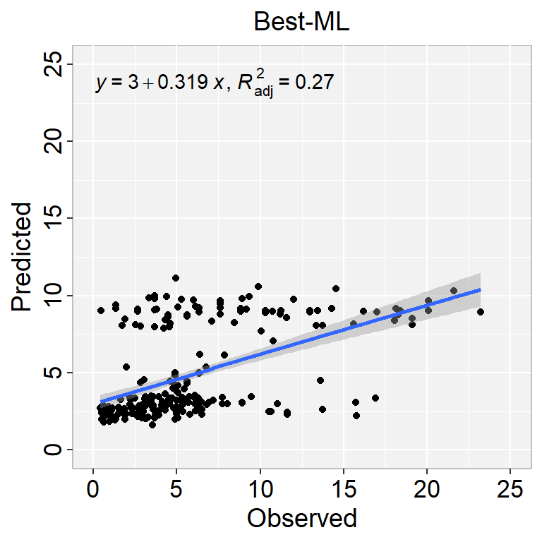
rmsle                     0.224472    0.285990    0.227318

Prediction

Code

best.test<-as.data.frame(h2o.predict(object = best_ML, newdata = h_test))
test.xy$Pred_SOC<-best.test$predict

Code

RMSE<- Metrics::rmse(test.xy$SOC, test.xy$Pred_SOC)
MAE<- Metrics::mae(test.xy$SOC, test.xy$Pred_SOC)

# Print results
paste0("RMSE: ", round(RMSE,2))

[1] "RMSE: 4.35"

Code

paste0("MAE: ", round(MAE,2))

[1] "MAE: 3"

Code

library(ggpmisc)
formula<-y~x

ggplot(test.xy, aes(SOC,Pred_SOC)) +
  geom_point() +
  geom_smooth(method = "lm")+
  stat_poly_eq(use_label(c("eq", "adj.R2")), formula = formula) +
  ggtitle("Best-ML") +
  xlab("Observed") + ylab("Predicted") +
  scale_x_continuous(limits=c(0,25), breaks=seq(0, 25, 5))+ 
  scale_y_continuous(limits=c(0,25), breaks=seq(0, 25, 5)) +
  # Flip the bars
  theme(
    panel.background = element_rect(fill = "grey95",colour = "gray75",size = 0.5, linetype = "solid"),
    axis.line = element_line(colour = "grey"),
    plot.title = element_text(size = 14, hjust = 0.5),
    axis.title.x = element_text(size = 14),
    axis.title.y = element_text(size = 14),
    axis.text.x=element_text(size=13, colour="black"),
    axis.text.y=element_text(size=13,angle = 90,vjust = 0.5, hjust=0.5, colour='black'))