Code
library(tidyverse)
# define data folder
urlfile = "https://github.com//zia207/r-colab/raw/main/Data/USA/gp_soil_data.csv"
mf<-read_csv(url(urlfile))
Multiple Regression Analysis is a statistical method used to examine the relationship between a dependent variable and two or more independent variables. It extends the concept of simple linear regression, which involves studying the relationship between a dependent variable and a single independent variable. In multiple regression, the goal is to understand how multiple independent variables together influence the variation in the dependent variable.
In this exercise we will use gp_soil_data.csv, The data can be found here for download.
library(tidyverse)
# define data folder
urlfile = "https://github.com//zia207/r-colab/raw/main/Data/USA/gp_soil_data.csv"
mf<-read_csv(url(urlfile))We will develop MLR model with five continuous predictors (‘DEM’, ‘Slope’, ‘MAT’, ‘MAP’,‘NDVI’) to explain variability soil organic carbon.
# Create a data-frame
df<-mf %>% dplyr::select(SOC, DEM, Slope, MAT, MAP,NDVI)
# fit MLR model
mlr_01<-lm(SOC~DEM+Slope+MAT+MAP+NDVI, df)
summary(mlr_01)
Call:
lm(formula = SOC ~ DEM + Slope + MAT + MAP + NDVI, data = df)

Residuals:
     Min       1Q   Median       3Q      Max
-13.5216  -2.1087  -0.4608   1.3395  16.3788

Coefficients:
              Estimate Std. Error t value Pr(>|t|)
(Intercept)  2.2088309  1.8002202   1.227 0.220457
DEM         -0.0003853  0.0005465  -0.705 0.481201
Slope        0.1660845  0.0632881   2.624 0.008972 **
MAT         -0.3239459  0.0821817  -3.942 9.34e-05 ***
MAP          0.0061026  0.0016366   3.729 0.000216 ***
NDVI         8.6687410  2.0697085   4.188 3.37e-05 ***
---
Signif. codes:  0 '***' 0.001 '**' 0.01 '*' 0.05 '.' 0.1 ' ' 1

Residual standard error: 3.812 on 461 degrees of freedom
Multiple R-squared:  0.4354,    Adjusted R-squared:  0.4293
F-statistic: 71.09 on 5 and 461 DF, p-value: < 2.2e-16We can create a regression summary table with tidy() function from the broom and stargazer() function from stargazer packages.
library(broom)
broom::tidy(mlr_01)
# A tibble: 6 × 5
term estimate std.error statistic p.value
<chr> <dbl> <dbl> <dbl> <dbl>
1 (Intercept) 2.21 1.80 1.23 0.220
2 DEM -0.000385 0.000547 -0.705 0.481
3 Slope 0.166 0.0633 2.62 0.00897
4 MAT -0.324 0.0822 -3.94 0.0000934
5 MAP 0.00610 0.00164 3.73 0.000216
6 NDVI 8.67 2.07 4.19 0.0000337library(stargazer)
stargazer::stargazer(mlr_01,type="text")
===============================================
                        Dependent variable:
                    ---------------------------
                                SOC
-----------------------------------------------
DEM                           -0.0004
                              (0.001)

Slope                        0.166***
                              (0.063)

MAT                          -0.324***
                              (0.082)

MAP                          0.006***
                              (0.002)

NDVI                         8.669***
                              (2.070)

Constant                       2.209
                              (1.800)

-----------------------------------------------
Observations                    467
R2                             0.435
Adjusted R2                    0.429
Residual Std. Error      3.812 (df = 461)
F Statistic           71.094*** (df = 5; 461)
===============================================
Note: *p<0.1; **p<0.05; ***p<0.01We can generate report for linear model using report() function of report package:
install.package(“report”)
library(report)
report::report(mlr_01)
We fitted a linear model (estimated using OLS) to predict SOC with DEM, Slope,
MAT, MAP and NDVI (formula: SOC ~ DEM + Slope + MAT + MAP + NDVI). The model
explains a statistically significant and substantial proportion of variance (R2
= 0.44, F(5, 461) = 71.09, p < .001, adj. R2 = 0.43). The model's intercept,
corresponding to DEM = 0, Slope = 0, MAT = 0, MAP = 0 and NDVI = 0, is at 2.21
(95% CI [-1.33, 5.75], t(461) = 1.23, p = 0.220). Within this model:
- The effect of DEM is statistically non-significant and negative (beta =
-3.85e-04, 95% CI [-1.46e-03, 6.89e-04], t(461) = -0.70, p = 0.481; Std. beta =
-0.06, 95% CI [-0.22, 0.11])
- The effect of Slope is statistically significant and positive (beta = 0.17,
95% CI [0.04, 0.29], t(461) = 2.62, p = 0.009; Std. beta = 0.15, 95% CI [0.04,
0.27])
- The effect of MAT is statistically significant and negative (beta = -0.32,
95% CI [-0.49, -0.16], t(461) = -3.94, p < .001; Std. beta = -0.26, 95% CI
[-0.39, -0.13])
- The effect of MAP is statistically significant and positive (beta = 6.10e-03,
95% CI [2.89e-03, 9.32e-03], t(461) = 3.73, p < .001; Std. beta = 0.25, 95% CI
[0.12, 0.38])
- The effect of NDVI is statistically significant and positive (beta = 8.67,
95% CI [4.60, 12.74], t(461) = 4.19, p < .001; Std. beta = 0.28, 95% CI [0.15,
0.41])
Standardized parameters were obtained by fitting the model on a standardized
version of the dataset. 95% Confidence Intervals (CIs) and p-values were
computed using a Wald t-distribution approximation.library(performance)
performance::model_performance(mlr_01)# Indices of model performance
AIC | AICc | BIC | R2 | R2 (adj.) | RMSE | Sigma
------------------------------------------------------------------
2583.012 | 2583.256 | 2612.037 | 0.435 | 0.429 | 3.787 | 3.812#| fig.width: 6
#| fig.height: 8
performance::check_model(mlr_01)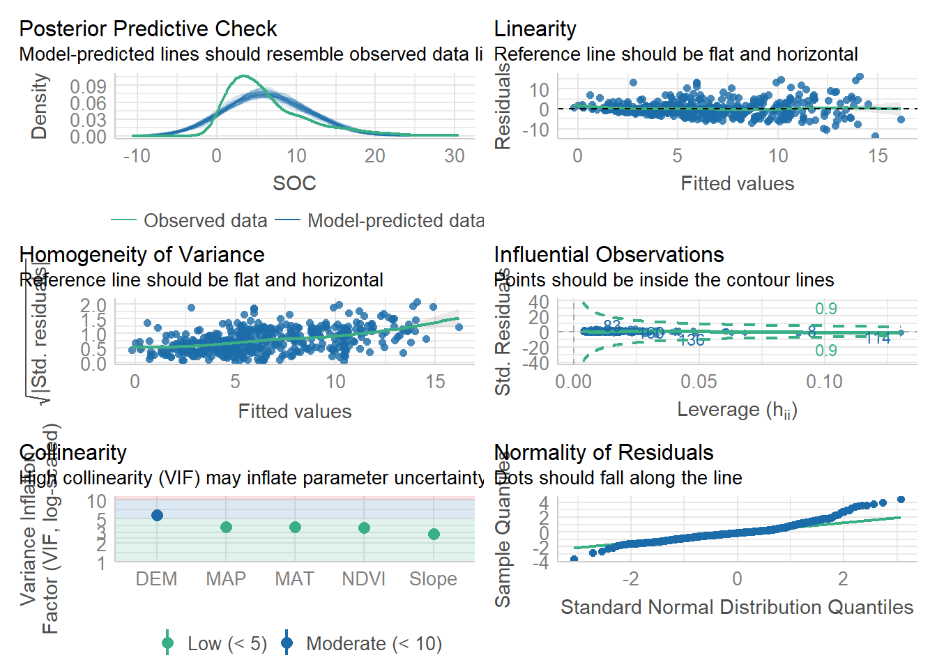
Now we will update the MLR model by adding tow categorical variables.
# Create a data-frame
df_02<-mf %>% dplyr::select(SOC, DEM, Slope, MAT, MAP,NDVI, NLCD, FRG)
# fit MLR model
mlr_02<-lm(SOC~DEM+Slope+MAT+MAP+NDVI+NLCD+FRG, df_02)stargazer::stargazer(mlr_02,type="text")
====================================================
                             Dependent variable:
                         ---------------------------
                                     SOC
----------------------------------------------------
DEM                                -0.0004
                                   (0.001)

Slope                              0.155**
                                   (0.069)

MAT                               -0.400***
                                   (0.101)

MAP                               0.007***
                                   (0.002)

NDVI                              6.828***
                                   (2.452)

NLCDHerbaceous                     -1.468*
                                   (0.880)

NLCDPlanted/Cultivated             -1.698*
                                   (0.990)

NLCDShrubland                      -1.161
                                   (0.798)

FRGFire Regime Group II           2.897***
                                   (1.038)

FRGFire Regime Group III            1.582
                                   (1.001)

FRGFire Regime Group IV             1.131
                                   (1.134)

FRGFire Regime Group V              0.957
                                   (1.391)

FRGIndeterminate FRG                1.789
                                   (1.739)

Constant                            2.529
                                   (2.832)

----------------------------------------------------
Observations                         467
R2                                  0.451
Adjusted R2                         0.436
Residual Std. Error           3.790 (df = 453)
F Statistic               28.669*** (df = 13; 453)
====================================================
Note: *p<0.1; **p<0.05; ***p<0.01report::report(mlr_02)We fitted a linear model (estimated using OLS) to predict SOC with DEM, Slope,
MAT, MAP, NDVI, NLCD and FRG (formula: SOC ~ DEM + Slope + MAT + MAP + NDVI +
NLCD + FRG). The model explains a statistically significant and substantial
proportion of variance (R2 = 0.45, F(13, 453) = 28.67, p < .001, adj. R2 =
0.44). The model's intercept, corresponding to DEM = 0, Slope = 0, MAT = 0, MAP
= 0, NDVI = 0, NLCD = Forest and FRG = Fire Regime Group I, is at 2.53 (95% CI
[-3.04, 8.09], t(453) = 0.89, p = 0.372). Within this model:
- The effect of DEM is statistically non-significant and negative (beta =
-4.48e-04, 95% CI [-1.79e-03, 8.92e-04], t(453) = -0.66, p = 0.511; Std. beta =
-0.07, 95% CI [-0.27, 0.14])
- The effect of Slope is statistically significant and positive (beta = 0.16,
95% CI [0.02, 0.29], t(453) = 2.27, p = 0.024; Std. beta = 0.14, 95% CI [0.02,
0.27])
- The effect of MAT is statistically significant and negative (beta = -0.40,
95% CI [-0.60, -0.20], t(453) = -3.98, p < .001; Std. beta = -0.33, 95% CI
[-0.49, -0.16])
- The effect of MAP is statistically significant and positive (beta = 6.76e-03,
95% CI [3.26e-03, 0.01], t(453) = 3.80, p < .001; Std. beta = 0.28, 95% CI
[0.13, 0.42])
- The effect of NDVI is statistically significant and positive (beta = 6.83,
95% CI [2.01, 11.65], t(453) = 2.78, p = 0.006; Std. beta = 0.22, 95% CI [0.06,
0.37])
- The effect of NLCD [Herbaceous] is statistically non-significant and negative
(beta = -1.47, 95% CI [-3.20, 0.26], t(453) = -1.67, p = 0.096; Std. beta =
-0.29, 95% CI [-0.63, 0.05])
- The effect of NLCD [Planted/Cultivated] is statistically non-significant and
negative (beta = -1.70, 95% CI [-3.64, 0.25], t(453) = -1.72, p = 0.087; Std.
beta = -0.34, 95% CI [-0.72, 0.05])
- The effect of NLCD [Shrubland] is statistically non-significant and negative
(beta = -1.16, 95% CI [-2.73, 0.41], t(453) = -1.46, p = 0.146; Std. beta =
-0.23, 95% CI [-0.54, 0.08])
- The effect of FRG [Fire Regime Group II] is statistically significant and
positive (beta = 2.90, 95% CI [0.86, 4.94], t(453) = 2.79, p = 0.005; Std. beta
= 0.57, 95% CI [0.17, 0.98])
- The effect of FRG [Fire Regime Group III] is statistically non-significant
and positive (beta = 1.58, 95% CI [-0.39, 3.55], t(453) = 1.58, p = 0.115; Std.
beta = 0.31, 95% CI [-0.08, 0.70])
- The effect of FRG [Fire Regime Group IV] is statistically non-significant and
positive (beta = 1.13, 95% CI [-1.10, 3.36], t(453) = 1.00, p = 0.319; Std.
beta = 0.22, 95% CI [-0.22, 0.67])
- The effect of FRG [Fire Regime Group V] is statistically non-significant and
positive (beta = 0.96, 95% CI [-1.78, 3.69], t(453) = 0.69, p = 0.492; Std.
beta = 0.19, 95% CI [-0.35, 0.73])
- The effect of FRG [Indeterminate FRG] is statistically non-significant and
positive (beta = 1.79, 95% CI [-1.63, 5.21], t(453) = 1.03, p = 0.304; Std.
beta = 0.35, 95% CI [-0.32, 1.03])
Standardized parameters were obtained by fitting the model on a standardized
version of the dataset. 95% Confidence Intervals (CIs) and p-values were
computed using a Wald t-distribution approximation.performance::model_performance(mlr_02)# Indices of model performance
AIC | AICc | BIC | R2 | R2 (adj.) | RMSE | Sigma
------------------------------------------------------------------
2585.591 | 2586.655 | 2647.786 | 0.451 | 0.436 | 3.733 | 3.790The compare_performance() function can be used to compare the performance and quality of several models (including models of different types). We can easily compute and a composite index of model performance and sort the models from the best one to the worse.
performance::compare_performance(mlr_01, mlr_02, rank = TRUE)# Comparison of Model Performance Indices
Name | Model | R2 | R2 (adj.) | RMSE | Sigma | AIC weights | AICc weights | BIC weights | Performance-Score
-----------------------------------------------------------------------------------------------------------------
mlr_02 | lm | 0.451 | 0.436 | 3.733 | 3.790 | 0.216 | 0.155 | 1.73e-08 | 57.14%
mlr_01 | lm | 0.435 | 0.429 | 3.787 | 3.812 | 0.784 | 0.845 | 1.000 | 42.86%Finally, we provide convenient visualization (the see package must be installed).
#| warning: false
#| error: false

#| fig.width: 4
#| fig.height: 4

plot(compare_performance(mlr_01, mlr_02, rank = TRUE))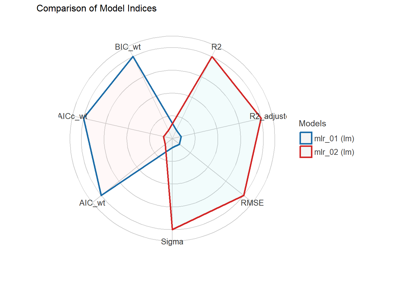
test_performance() and test_bf, carries out the most relevant and appropriate tests based on the input (for instance, whether the models are nested or not).
performance::test_performance(mlr_01, mlr_02)Name | Model | BF | df | df_diff | Chi2 | p
--------------------------------------------------------
mlr_01 | lm | | 7 | | |
mlr_02 | lm | 1.73e-08 | 15 | 8.00 | 13.42 | 0.098
Models were detected as nested and are compared in sequential order.#test_bf(mlr_01, mlr_02)Th “jtools” package consists of a series of functions to automate visualization regression model.

install.packages (“jtools”)
library(jtools)summ() is a replacement for summary() that provides the user several options for formatting regression summaries. It supports glm, svyglm, and merMod objects as input as well. It supports calculation and reporting of robust standard errors via the sandwich package.
jtools::summ(mlr_02)| Observations | 467 |
| Dependent variable | SOC |
| Type | OLS linear regression |
| F(13,453) | 28.67 |
| R² | 0.45 |
| Adj. R² | 0.44 |
| Est. | S.E. | t val. | p | |
|---|---|---|---|---|
| (Intercept) | 2.53 | 2.83 | 0.89 | 0.37 |
| DEM | -0.00 | 0.00 | -0.66 | 0.51 |
| Slope | 0.16 | 0.07 | 2.27 | 0.02 |
| MAT | -0.40 | 0.10 | -3.98 | 0.00 |
| MAP | 0.01 | 0.00 | 3.80 | 0.00 |
| NDVI | 6.83 | 2.45 | 2.78 | 0.01 |
| NLCDHerbaceous | -1.47 | 0.88 | -1.67 | 0.10 |
| NLCDPlanted/Cultivated | -1.70 | 0.99 | -1.72 | 0.09 |
| NLCDShrubland | -1.16 | 0.80 | -1.46 | 0.15 |
| FRGFire Regime Group II | 2.90 | 1.04 | 2.79 | 0.01 |
| FRGFire Regime Group III | 1.58 | 1.00 | 1.58 | 0.11 |
| FRGFire Regime Group IV | 1.13 | 1.13 | 1.00 | 0.32 |
| FRGFire Regime Group V | 0.96 | 1.39 | 0.69 | 0.49 |
| FRGIndeterminate FRG | 1.79 | 1.74 | 1.03 | 0.30 |
| Standard errors: OLS |
You can also get variance inflation factors (VIFs) and partial/semipartial (AKA part) correlations. Partial correlations are only available for OLS models. You may also substitute confidence intervals in place of standard errors and you can choose whether to show p values.
jtools::summ(mlr_02,
     scale = TRUE,
     vifs = TRUE,
     part.corr = TRUE,
     confint = TRUE,
pvals = FALSE)| Observations | 467 |
| Dependent variable | SOC |
| Type | OLS linear regression |
| F(13,453) | 28.67 |
| R² | 0.45 |
| Adj. R² | 0.44 |
| Est. | 2.5% | 97.5% | t val. | VIF | partial.r | part.r | |
|---|---|---|---|---|---|---|---|
| (Intercept) | 5.36 | 3.41 | 7.31 | 5.40 | NA | NA | NA |
| DEM | -0.34 | -1.38 | 0.69 | -0.66 | 8.94 | -0.03 | -0.02 |
| Slope | 0.73 | 0.10 | 1.36 | 2.27 | 3.37 | 0.11 | 0.08 |
| MAT | -1.64 | -2.45 | -0.83 | -3.98 | 5.53 | -0.18 | -0.14 |
| MAP | 1.40 | 0.68 | 2.12 | 3.80 | 4.40 | 0.18 | 0.13 |
| NDVI | 1.11 | 0.33 | 1.89 | 2.78 | 5.11 | 0.13 | 0.10 |
| NLCDHerbaceous | -1.47 | -3.20 | 0.26 | -1.67 | 9.63 | -0.08 | -0.06 |
| NLCDPlanted/Cultivated | -1.70 | -3.64 | 0.25 | -1.72 | 9.63 | -0.08 | -0.06 |
| NLCDShrubland | -1.16 | -2.73 | 0.41 | -1.46 | 9.63 | -0.07 | -0.05 |
| FRGFire Regime Group II | 2.90 | 0.86 | 4.94 | 2.79 | 8.60 | 0.13 | 0.10 |
| FRGFire Regime Group III | 1.58 | -0.39 | 3.55 | 1.58 | 8.60 | 0.07 | 0.05 |
| FRGFire Regime Group IV | 1.13 | -1.10 | 3.36 | 1.00 | 8.60 | 0.05 | 0.03 |
| FRGFire Regime Group V | 0.96 | -1.78 | 3.69 | 0.69 | 8.60 | 0.03 | 0.02 |
| FRGIndeterminate FRG | 1.79 | -1.63 | 5.21 | 1.03 | 8.60 | 0.05 | 0.04 |
| Standard errors: OLS; Continuous predictors are mean-centered and scaled by 1 s.d. The outcome variable remains in its original units. |
Variance Inflation factors (VIFs): Variance inflation factors (VIFs) are a measure of multicollinearity in regression analysis. Multicollinearity occurs when two or more independent variables in a regression model are highly correlated, which can lead to unreliable estimates of the regression coefficients.
VIF is calculated for each independent variable in the regression model, and it represents the extent to which that variable’s variance is inflated by the presence of other independent variables in the model. Specifically, VIF measures the ratio of the variance of the coefficient estimate for a particular independent variable in a model that includes all the independent variables, to the variance of the coefficient estimate for that same variable in a model that includes only that variable and the constant.
A VIF of 1 indicates that there is no multicollinearity between the independent variable and the other variables in the model. Generally, a VIF greater than 5 or 10 is considered high, indicating that multicollinearity is a potential issue.
Partial/semipartial (AKA part) correlations: Partial or semipartial (also known as part) correlations are a statistical technique used to determine the degree of association between two variables while controlling for the effects of one or more additional variables.
Partial correlations measure the association between two variables, while controlling for the effects of other variables in the analysis. It calculates the correlation coefficient between two variables while holding all other variables constant. Partial correlation is used to determine the unique contribution of each variable in the relationship between two other variables.
Semipartial correlations, on the other hand, measure the degree of association between two variables while controlling for the effects of one additional variable. It is also known as a part correlation, as it quantifies the unique variance that a particular independent variable explains in the dependent variable, after controlling for the other independent variables in the analysis.
Partial and semipartial correlations are useful in situations where two or more variables are highly correlated, and it is difficult to determine their individual effects on the dependent variable. By controlling for the effects of other variables, these correlations can provide a more accurate estimate of the strength of the relationship between two variables. They are commonly used in regression analysis, where the goal is to determine the unique contribution of each independent variable in predicting the dependent variable.
Sometimes the best way to understand your model is to look at the predictions it generates. Rather than look at coefficients, effect_plot() lets you plot predictions across values of a predictor variable alongside the observed data.
And a new feature in version 2.0.0 lets you plot partial residuals instead of the raw observed data, allowing you to assess model quality after accounting for effects of control variables.
jtools::effect_plot(mlr_02, pred = NDVI, interval = TRUE, partial.residuals = TRUE)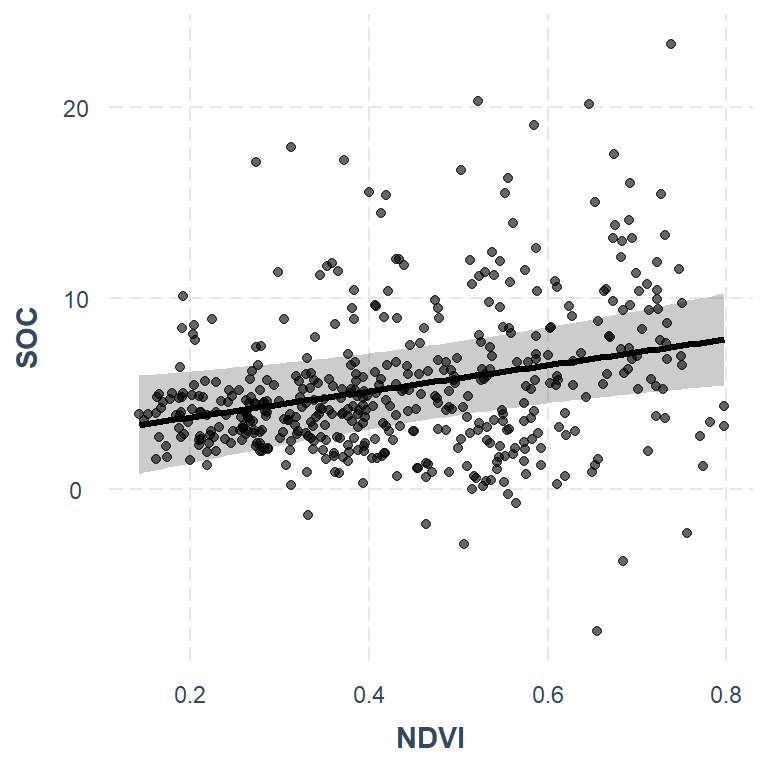
jtools::effect_plot(mlr_02, pred =NLCD, interval = TRUE)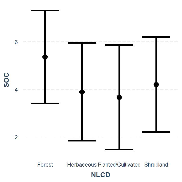
The relaimpo package provides measures of relative importance for each of the predictors in the model. See help(calc.relimp) for details on the four measures of relative importance provided.
install.package(“relaimpo”)
#| fig.width: 8
#| fig.height: 8

# Calculate Relative Importance for Each Predictor
library(relaimpo)
rvip<-calc.relimp(mlr_01,
                 type = c("lmg", "last", "first", "betasq", "pratt", "car"),
                 rela=TRUE)
plot(rvip)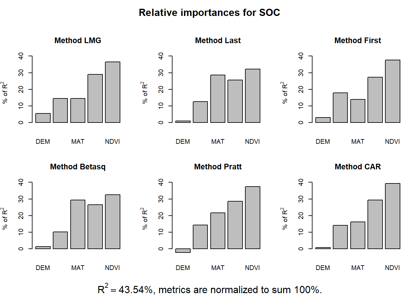
lmg: is the R2 contribution averaged over orderings among regressors, cf. e.g. Lindeman, Merenda and Gold 1980, p.119ff or Chevan and Sutherland (1991).
pmvd: is the proportional marginal variance decomposition as proposed by Feldman (2005) (non-US version only). It can be interpreted as a weighted average over orderings among regressors, with data-dependent weights.
last: is each variables contribution when included last, also sometimes called usefulness.
first: is each variables contribution when included first, which is just the squared covariance between y and the variable.
betasq: is the squared standardized coefficient.
pratt: is the product of the standardized coefficient and the correlation.
genizi: is the R2 decomposition according to Genizi 1993
car: is the R2 decomposition according to Zuber and Strimmer 2010, also available from package care (squares of scores produced by function carscore