Working with Raster Data in R

Raster data processing in R is commonly done using packages such as raster and rgdal. Raster data consists of grids of cells, where each cell holds a value representing some information, such as elevation, temperature, or land cover type. The raster package provides functions for reading, manipulating, and analyzing raster data, while the rgdal package focuses on reading and writing geospatial raster data formats.

The terra package is an advanced geospatial package in R that provides powerful tools for working with raster data. It is designed to handle large datasets efficiently and offers a wide range of capabilities for raster data processing, analysis, and visualization. terra is considered a successor to the raster package and aims to provide better performance and support for more complex operations.

Here are some key features and concepts of the terra package:

Efficiency and Performance: terra is optimized for performance, making it suitable for processing large raster datasets. It leverages modern computing hardware and parallel processing capabilities to efficiently handle computations.
Raster Objects: terra introduces the concept of “SpatioTemporalRaster” objects, which are used to represent raster data along with its spatial and temporal attributes.
Basic Operations: Similar to the raster package, terra allows you to perform basic operations like reading, writing, displaying, and extracting values from raster data.
Spatial and Temporal Operations: terra supports spatial and temporal operations such as cropping, reprojecting, resampling, masking, and aggregating raster data. It also handles multi-layer raster stacks efficiently.
Advanced Analytics: The package provides functions for more advanced spatial analytics, including focal operations (neighborhood analysis), zonal statistics, and mathematical operations on raster layers.
Memory Management: terra uses a “lazy” evaluation approach, which means that computations are performed only when needed. This allows for more memory-efficient processing of large datasets.
Visualization: The package includes visualization functions to help you create maps and plots of raster data.
Integration with Other Packages: terra can be integrated with other geospatial packages like sf for vector data handling and analysis.

In this exerciser we will learn following raster processing techniques with R:

Basic Raster Operation
Clipping
Reclassification
Focal Statistics
Raster Algebra
Aggregation
Disaggregation
Resample
Mosaic
Vector to raster conversion
- Convert Raster to Point Data
- Convert Point Data to Raster
Raster Stack and Raster Brick

Load R packages

Code

library (terra)           
library(sf)       
library (rgdal)     
library(tidyverse)
library(rgeos)
library(maptools)
library(classInt)     
library(RColorBrewer)   
library(raster)

Data

We will use SRTM elevation data (250 m x 250 m) of all hilly districts of Bangladesh and The data can be found here for download.

We will use rast() function of terra package to load raster in R

Code

dataFolder<-"G:\\My Drive\\Data\\Bangladesh\\"
# if data in working directory
dem<-terra::rast(paste0(dataFolder, "/Raster/hilly_DEM_UTM.tif"))

We can load data from github:

Code

dem= terra::rast("/vsicurl/https://github.com//zia207/r-colab/raw/main/Data/Bangladesh/Raster/hilly_DEM_UTM.tif")

You can also load data with raster packages, but raster object relatively slow to perform some tasks. The terra library is more recent (but faster). We can convert a RasterLayer (i.e. a raster object) into a SpatRaster (i.e. a terra object):

Code

dem.r<-raster::raster(paste0(dataFolder, "/Raster/hilly_DEM_UTM.tif"))
dem.r

class      : RasterLayer 
dimensions : 1329, 521, 692409  (nrow, ncol, ncell)
resolution : 250, 250  (x, y)
extent     : 648050.4, 778300.4, 2295017, 2627267  (xmin, xmax, ymin, ymax)
crs        : +proj=tmerc +lat_0=0 +lon_0=90 +k=0.9996 +x_0=500000 +y_0=0 +datum=WGS84 +units=m +no_defs 
source     : hilly_DEM_UTM.tif 
names      : Band_1 
values     : -7.796429, 985.0496  (min, max)

Code

# terra object
dem.t<-as(dem.r, "SpatRaster")
dem.t

class       : SpatRaster 
dimensions  : 1329, 521, 1  (nrow, ncol, nlyr)
resolution  : 250, 250  (x, y)
extent      : 648050.4, 778300.4, 2295017, 2627267  (xmin, xmax, ymin, ymax)
coord. ref. : +proj=tmerc +lat_0=0 +lon_0=90 +k=0.9996 +x_0=500000 +y_0=0 +datum=WGS84 +units=m +no_defs 
source      : hilly_DEM_UTM.tif 
name        :     Band_1 
min value   :  -7.796429 
max value   : 985.049622

Basic Raster Operation

Check projection system

Code

crs(dem, parse = TRUE)

 [1] "PROJCRS[\"WGS_1984_Transverse_Mercator\","                   
 [2] "    BASEGEOGCRS[\"WGS 84\","                                 
 [3] "        DATUM[\"World Geodetic System 1984\","               
 [4] "            ELLIPSOID[\"WGS 84\",6378137,298.257223563,"     
 [5] "                LENGTHUNIT[\"metre\",1]]],"                  
 [6] "        PRIMEM[\"Greenwich\",0,"                             
 [7] "            ANGLEUNIT[\"degree\",0.0174532925199433]],"      
 [8] "        ID[\"EPSG\",4326]],"                                 
 [9] "    CONVERSION[\"Transverse Mercator\","                     
[10] "        METHOD[\"Transverse Mercator\","                     
[11] "            ID[\"EPSG\",9807]],"                             
[12] "        PARAMETER[\"Latitude of natural origin\",0,"         
[13] "            ANGLEUNIT[\"degree\",0.0174532925199433],"       
[14] "            ID[\"EPSG\",8801]],"                             
[15] "        PARAMETER[\"Longitude of natural origin\",90,"       
[16] "            ANGLEUNIT[\"degree\",0.0174532925199433],"       
[17] "            ID[\"EPSG\",8802]],"                             
[18] "        PARAMETER[\"Scale factor at natural origin\",0.9996,"
[19] "            SCALEUNIT[\"unity\",1],"                         
[20] "            ID[\"EPSG\",8805]],"                             
[21] "        PARAMETER[\"False easting\",500000,"                 
[22] "            LENGTHUNIT[\"metre\",1],"                        
[23] "            ID[\"EPSG\",8806]],"                             
[24] "        PARAMETER[\"False northing\",0,"                     
[25] "            LENGTHUNIT[\"metre\",1],"                        
[26] "            ID[\"EPSG\",8807]]],"                            
[27] "    CS[Cartesian,2],"                                        
[28] "        AXIS[\"easting\",east,"                              
[29] "            ORDER[1],"                                       
[30] "            LENGTHUNIT[\"metre\",1,"                         
[31] "                ID[\"EPSG\",9001]]],"                        
[32] "        AXIS[\"northing\",north,"                            
[33] "            ORDER[2],"                                       
[34] "            LENGTHUNIT[\"metre\",1,"                         
[35] "                ID[\"EPSG\",9001]]]]"

Check raster attribute

Code

dem

class       : SpatRaster 
dimensions  : 1329, 521, 1  (nrow, ncol, nlyr)
resolution  : 250, 250  (x, y)
extent      : 648050.4, 778300.4, 2295017, 2627267  (xmin, xmax, ymin, ymax)
coord. ref. : WGS_1984_Transverse_Mercator 
source      : hilly_DEM_UTM.tif 
name        :     Band_1 
min value   :  -7.796429 
max value   : 985.049622

Raster extent

Code

ext(dem)

SpatExtent : 648050.374681405, 778300.374681405, 2295017.2625413, 2627267.2625413 (xmin, xmax, ymin, ymax)

Raster statistics

R allow you to calculate some basic statistics of raster data. We can use summary function to get some statistics of raster layer.

Code

summary(dem)

     Band_1      
 Min.   : -5.92  
 1st Qu.: 29.36  
 Median : 64.96  
 Mean   :108.99  
 3rd Qu.:137.46  
 Max.   :956.86  
 NA's   :55264

Histogram of raster

R-base function hist() is also useful to know frequency of raster values

Code

HISTO.DEM<-hist(dem,    
     breaks=6,  
     col= "purple",                                              # color of histogram 
     main="Distribution of Elevation values with 5 breaks",     # tittle of the plot
     xlab= "Elevation (m)",                                     # x-axis name
     ylab = "Number of Pixels")                                 # y-axis name
box()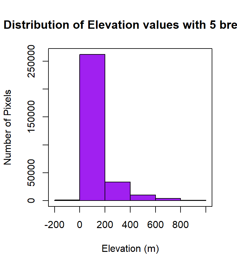

Plot raster

We can plot raster in diffrent ways in R. R base function plot() can easily apply on raster object for visualization:

Code

plot(dem, main="DEM of  Hilly District of Bangladesh")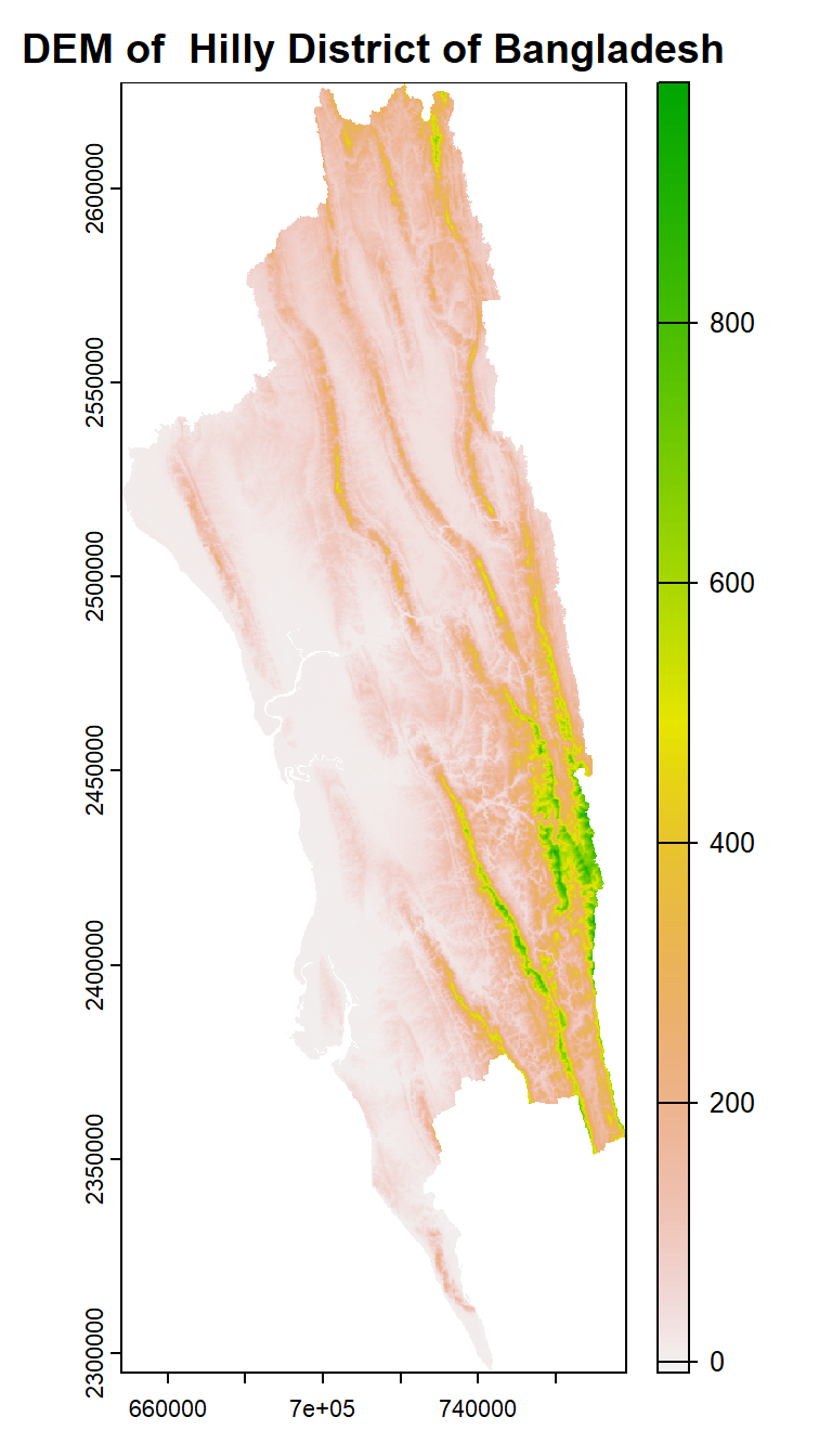

R has an image() function that allows you to control the way a raster is rendered on the screen. The plot() function in R has a base setting for the number of pixels that it will plot (100,000 pixels). The image command thus might be better for rendering larger rasters.

Code

image(dem)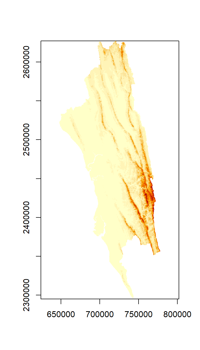

To visualize raster in R using ggplot2, first we need to convert it to a dataframe. The terra package has an built-in function for conversion to a plotable dataframe. Then we can applly geom_raster() of ggplot().

Code

dem.df <- as.data.frame(dem, xy = TRUE)%>%
  glimpse()

Rows: 310,665
Columns: 3
$ x      <dbl> 720925.4, 720175.4, 720425.4, 720675.4, 720925.4, 721175.4, 719…
$ y      <dbl> 2627142, 2626892, 2626892, 2626892, 2626892, 2626892, 2626642, …
$ Band_1 <dbl> 357.0371, 318.1637, 320.6357, 317.4960, 355.9710, 440.9489, 251…

Code

dem %>% as.data.frame(xy = TRUE) %>%
ggplot() +
    geom_raster(aes(x = x, y = y, fill = Band_1)) +
    scale_fill_viridis_c() +
    coord_quickmap()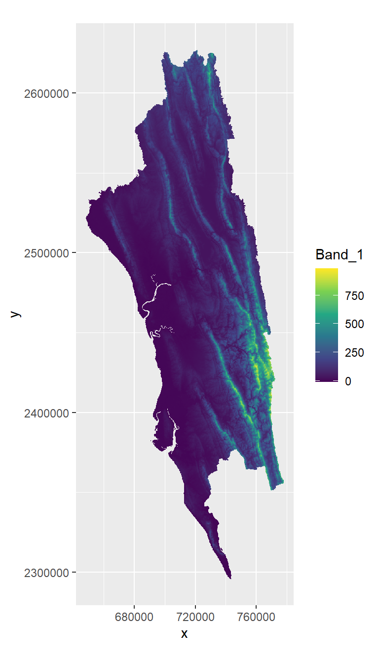

Clipping

Raster clipping refers to the process of extracting a portion of a raster dataset based on a specified spatial extent or boundary. This is a common operation in geospatial analysis when you need to focus on a specific area of interest within a larger raster dataset. Raster clipping can help reduce the dataset’s size, improve processing efficiency, and facilitate analysis that’s relevant to a particular region.

In R, you can perform raster clipping using various packages, including raster, terra, and others. I’ll provide examples using both the raster and terra packages.

In this exercise, we will clip hilly area DEM with extent of Bandarban district shape file. First we have to create a shape file of this district:

Code

bd.dist = sf::st_read("/vsicurl/https://github.com//zia207/r-colab/raw/main/Data/Bangladesh//Shapefiles//bd_district_BTM.shp")

Reading layer `bd_district_BTM' from data source 
  `/vsicurl/https://github.com//zia207/r-colab/raw/main/Data/Bangladesh//Shapefiles//bd_district_BTM.shp' 
  using driver `ESRI Shapefile'
Simple feature collection with 64 features and 14 fields
Geometry type: MULTIPOLYGON
Dimension:     XY
Bounding box:  xmin: 298487.8 ymin: 278578.1 xmax: 778101.8 ymax: 946939.2
Projected CRS: +proj=tmerc +lat_0=0 +lon_0=90 +k=0.9996 +x_0=500000 +y_0=-2000000 +datum=WGS84 +units=m +no_defs

Code

bandarban.dist = bd.dist %>%
  rename(DIST_Name = ADM2_EN) %>%
  filter(DIST_Name == "Bandarban")

Before clipping, you have to make sure both raster and vector data are in same projection systems.

Code

identical(crs(dem), crs(bandarban.dist ))

[1] FALSE

It looks like DEM in UTM and district shape files is BUTM project system. We have bring them in same projection system before clipping. Here we reproject DEM to BUTM using district shape files

Code

dem.BTM <- terra::project(dem, crs(bandarban.dist))
#terra::writeRaster(dem.BTM, paste0(dataFolder,"Raster/hilly_dem_BTM.tiff"), filetype = "GTiff", overwrite = TRUE)

Code

identical(crs(dem.BTM), crs(bandarban.dist ))

[1] TRUE

Code

plot(dem.BTM)
plot(bandarban.dist$geometry, add=TRUE)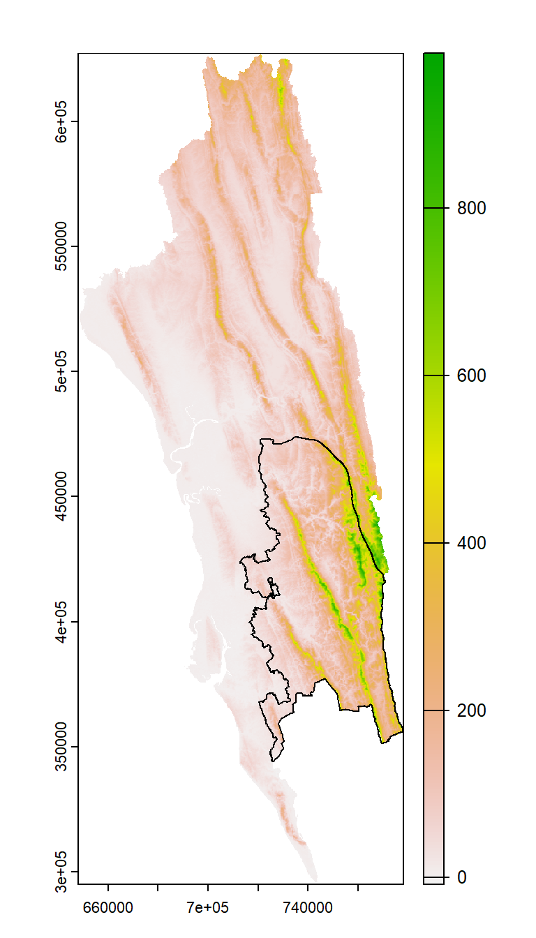

In R, clipping of a raster is two steps procedure, first you have to apply crop() function & then mask functions of raster package. crop returns a geographic subset of an object as specified by an extent object (or object from which an extent object can be extracted/created). mask Create a new Raster object that has the same values as input raster.

Code

bandarban.dem_01<- crop(dem.BTM, ext(bandarban.dist))
bandarban.dem_02<-mask(bandarban.dem_01, bandarban.dist)

Code

bandarban.dem_02 %>% as.data.frame(xy = TRUE) %>%
ggplot() +
    geom_raster(aes(x = x, y = y, fill = Band_1)) +
    scale_fill_viridis_c() +
    coord_quickmap()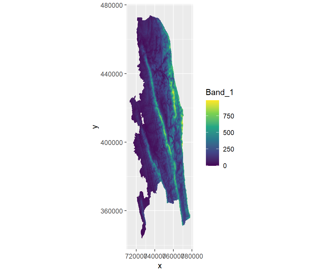

We can write raster using terra::writeRaster function:

Code

terra::writeRaster(bandarban.dem_02, paste0(dataFolder,"Raster/bandarban_dem_BTM.tiff"), filetype = "GTiff", overwrite = TRUE)
#terra::writeRaster(bandarban.dem, "/content/drive/MyDrive/Data/Bangladesh/Raster/bandarban_dem_BTM.tiff",filetype = "GTiff", overwrite = TRUE )

Reclassification

Raster reclassification is the process of assigning new values to the cells of a raster dataset based on predefined criteria. This operation is commonly used in geospatial analysis to reclassify continuous raster data (e.g., elevation, temperature) into discrete categories (e.g., low, medium, high).

In R, you can perform raster reclassification using packages like raster or terra packages

Histogram

Before reclassification, we will create a histogram with 5 breaks, of dem raster

Code

hist.dem<-hist(dem.BTM, 
     breaks=4,  
     col= "purple",                                             # color of histogram 
     main="Distribution of Elevation values with 5 breaks",     # tittle of the plot
     xlab= "Elevation (m)",                                     # x-axis name
     ylab = "Number of Pixels")                                 # y-axis name
box()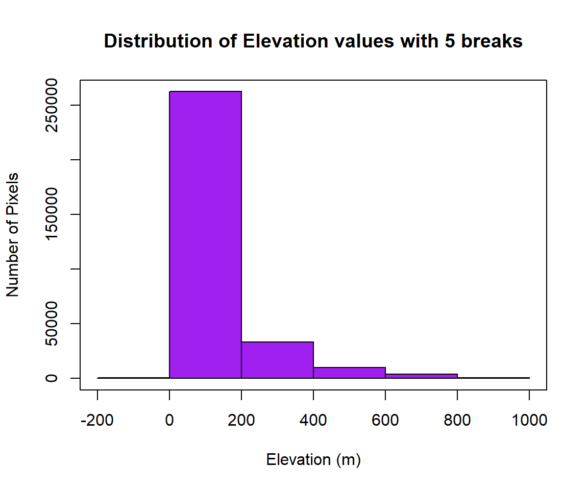

Now, you can check where are breaks and how many pixels in each category, and use these breaks to plot a raster layer

Code

hist.dem$breaks

[1] -200    0  200  400  600  800 1000

Code

hist.dem$counts

[1]    778 262373  33316  10008   3775    415

Code

# plot using  the histogram breaks.
plot(dem.BTM, 
     breaks = c(0, 200, 400, 600, 800, 1000), 
     col = terrain.colors(7),
     main="DEM ")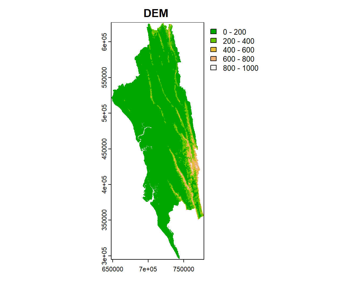

We will use following breaks of histogram to reclassify the dem raster. First, you have to create classification matrix

Class 1: -200 - 0 m (low elevation)
Class 2: 0 - 400 m (medium elevation)
Class 3: 400 - 1000 (Inf) m (high elevation)

Code

# Create a dataframe
reclass_df <- c(-200, 200, 1,
                200, 400, 2,
                400, Inf, 3)
reclass_df

[1] -200  200    1  200  400    2  400  Inf    3

Next, you have to reshape the data frame to matrix using matrix function

Code

reclass_m <- matrix(reclass_df,
                ncol = 3,
                byrow = TRUE)
reclass_m

     [,1] [,2] [,3]
[1,] -200  200    1
[2,]  200  400    2
[3,]  400  Inf    3

Now you have to apply terra::classify() function of raster package using re-class_m object.

Code

dem.reclass <-  terra::classify(dem.BTM,
                     reclass_m)

You can view the distribution of pixels assigned to each class using the bar-plot().

Code

barplot(dem.reclass,
        main = "Number of pixels in each class")
box()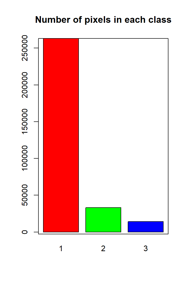

Now we plot the reclassified raster using plot function with a nice looking legend

Code

plot(dem.reclass,
     legend = FALSE,
     col = c("green", "blue", "red"), axes = FALSE,
     main = "Reclassified DEM")
legend("topright",
       legend = c("Low", "Medium", "High"),
       fill = c("green", "blue", "red"),
       border = FALSE,
       bty = "n") # turn off legend border
box()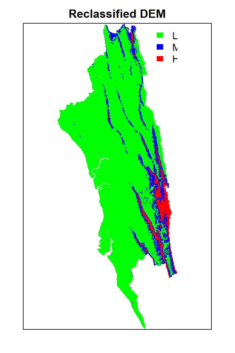

Quantile

If you want create a raster map using the quantile, you fave to use classInt package. The classIntervals function is create a custom breaks of raster values using different styles (such as “fixed”, “sd”, “equal”, “pretty”, “quantile”, “kmeans”, “hclust”, “bclust”, “fisher”, & “jenks”). For details, please see help, just type ?classIntervals in R console

First, we have to convert raster to vector using values function. Then, you have to create a object with a quantile interval applying classIntervals function to vector data.

Code

value.vector <- values(dem.BTM)
value.vector <- value.vector[value.vector != 0]
at = round(classIntervals(value.vector, n = 10, style = "quantile")$brks, 0) # 10 quantile
at

 [1]  -8   7  20  35  49  65  87 117 164 267 985

Now, we plot the DEM raster using the this custom break. We will use sppot function from sp package to plot raster data with state boundary shape file. Before that we will create a custom color palette using colorRampPalette of RColorBrewer.

Code

rgb.palette <- colorRampPalette(c("lightblue","blue","green","yellow","red"),
space = "rgb")
#polys<- list("sp.lines", as(dem, "SpatialLines"), col="grey", lty=1)  # CO state boundary
spplot(dem.BTM, main = "Quantile of DEM (m)",
   at=at,
   #sp.layout=list(polys),
   par.settings=list(axis.line=list(col="darkgrey",lwd=1)),
   colorkey=list(space="right",height=1, width=1.3,at=1:11,labels=list(cex=1.0,at=1:11,
   labels=c("-8","7","20","35","49","65","87","117","164","267","985"))),
   col.regions=rgb.palette(100))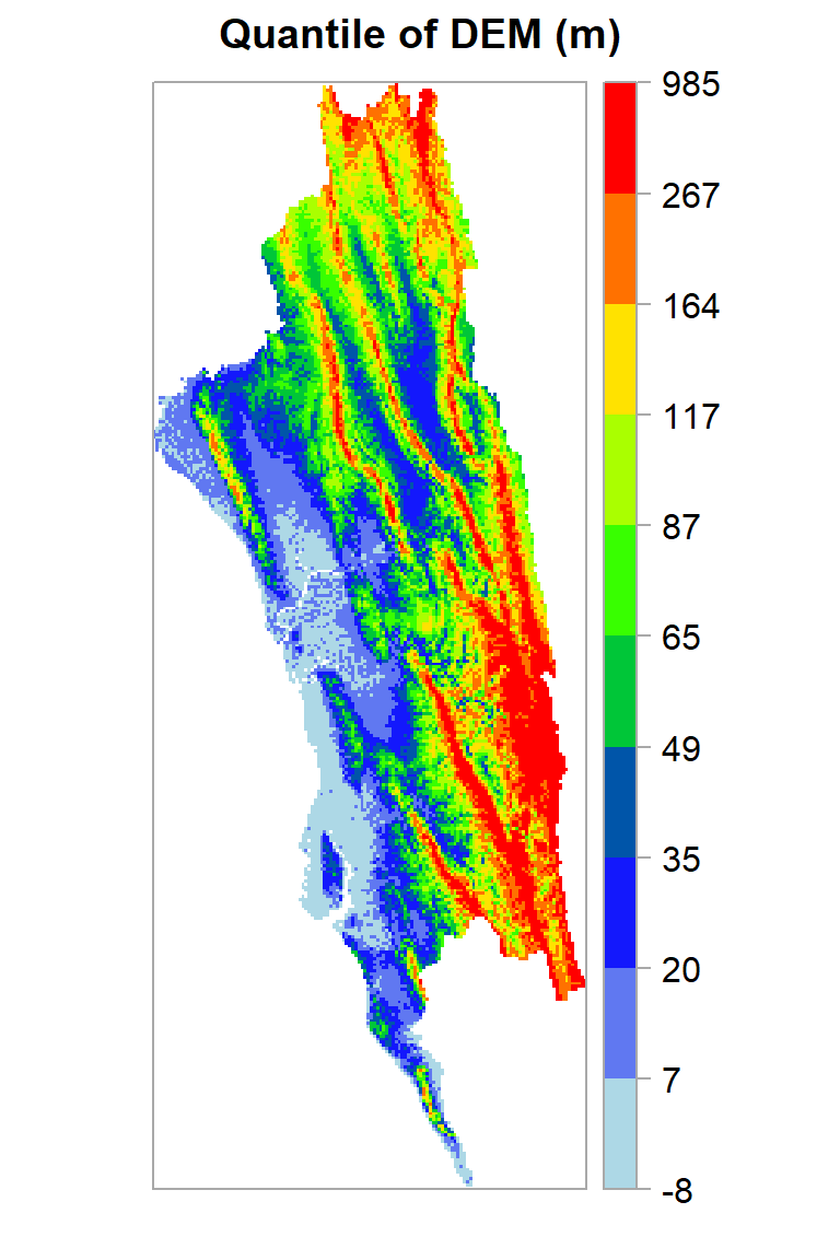

Focal Statistics

Focal statistics, also known as neighborhood or moving window statistics, involve performing calculations on a raster dataset using a moving window that slides over each cell. This window defines a local area around each cell, and calculations are carried out based on the values within that window. This technique is commonly used for various geospatial analysis tasks, such as smoothing, edge detection, and texture analysis.

In R, you can perform focal statistics using packages like raster and terra.

To illustrate the neighborhood processing for Focal Statistics calculating a Sum statistic, consider the processing cell with a value of 5 in the following diagram. A rectangular 3 by 3 cell neighborhood shape is specified. The sum of the values of the neighboring cells (3 + 2 + 3 + 4 + 2 + 1 + 4 = 19) plus the value of the processing cell (5) equals 24 (19 + 5 = 24). So a value of 24 is given to the cell in the output raster in the same location as the processing cell in the input raster.

The above figure demonstrates how the calculations are performed on a single cell in the input raster. In the following diagram, the results for all the input cells are shown. The cells highlighted in yellow identify the same processing cell and neighborhood as in the example above.

We will calculate focal mean of each cell of DEM data using focal() function of terra package.

Code

focal.sum<- focal(dem.BTM, 
    w=matrix(1/9,nrow=9,ncol=9),    # matrix of weights for 9 x 9 
    fun=sum)

Code

spplot(focal.sum, main="Focal Sum of DEM (m)")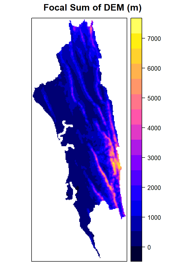

Code

focal.mean<- focal(dem.BTM, 
    w=matrix(1/9,nrow=9,ncol=9),    # matrix of weights for 3 x 3 
    fun=mean)

Code

spplot(focal.mean,main="Focal Mean of DEM (m)")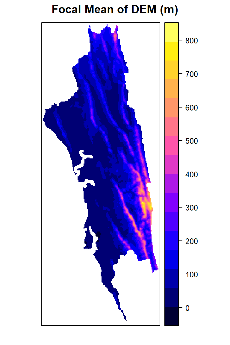

Raster Algebra

Raster algebra, also known as map algebra, involves performing mathematical operations on raster datasets to create new raster outputs. It’s a fundamental technique in geospatial analysis that allows you to combine, modify, and analyze raster data using various arithmetic and logical operations.

A simple sample of raster algebra in R is to convert unit of DEM raster from meter to feet (1 m = 3.28084 feet)

Code

dem.feet<-dem.BTM*3.28084
plot(dem.feet, main= "DEM (feet)")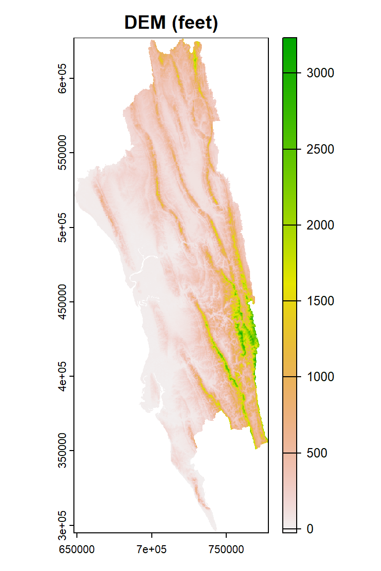

Code

dem.feet.1000<-dem.feet/1000
plot(dem.feet.1000, main = "DEM (feet x 1000)")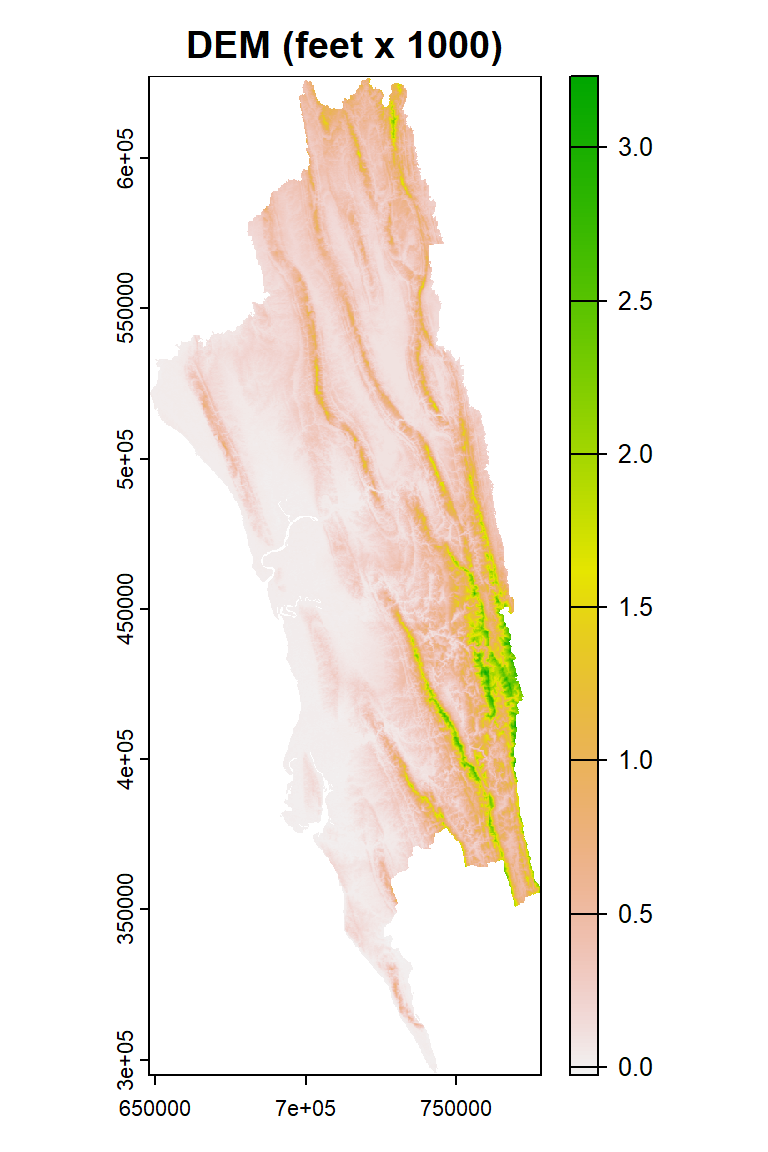

Aggregation

Raster aggregation involves converting a high-resolution raster dataset into a lower-resolution raster dataset by grouping or summarizing cells into larger cells. This process reduces the level of detail in the data and can help improve processing efficiency and visualization for large datasets. Aggregation is often used when working with raster data at different scales, or when matching the resolution of one raster to another for analysis or visualization purposes.

First, we will create 500 x 500 km raster (mean & standard deviation) from 250 m x 250 m raster using aggregate function of raster package. To achieve this, we can combine pixels 2 by 2 (horizontally and vertically) using the aggregate() function and the argument fact = 2.

Code

#rm(mean)
#rm(sd)
mean.DEM<-aggregate(dem.BTM, fact=2, fun=mean) 
sd.DEM<-aggregate(dem, fact=2, fun=sd) 
se.DEM<-sd.DEM/sqrt(2)
mean.DEM

class       : SpatRaster 
dimensions  : 665, 261, 1  (nrow, ncol, nlyr)
resolution  : 500, 500  (x, y)
extent      : 648050.4, 778550.4, 294767.3, 627267.3  (xmin, xmax, ymin, ymax)
coord. ref. : +proj=tmerc +lat_0=0 +lon_0=90 +k=0.9996 +x_0=500000 +y_0=-2000000 +datum=WGS84 +units=m +no_defs 
source(s)   : memory
name        :     Band_1 
min value   :  -4.500583 
max value   : 922.961380

Code

p1<-spplot(mean.DEM, main="500 m x 500 m of DEM")
p2<-spplot(sd.DEM, main="SD (m) ")
p3<-spplot(se.DEM, main="SE (m) )")

Code

library(gridExtra)
grid.arrange(p1, p2, p3, ncol=3)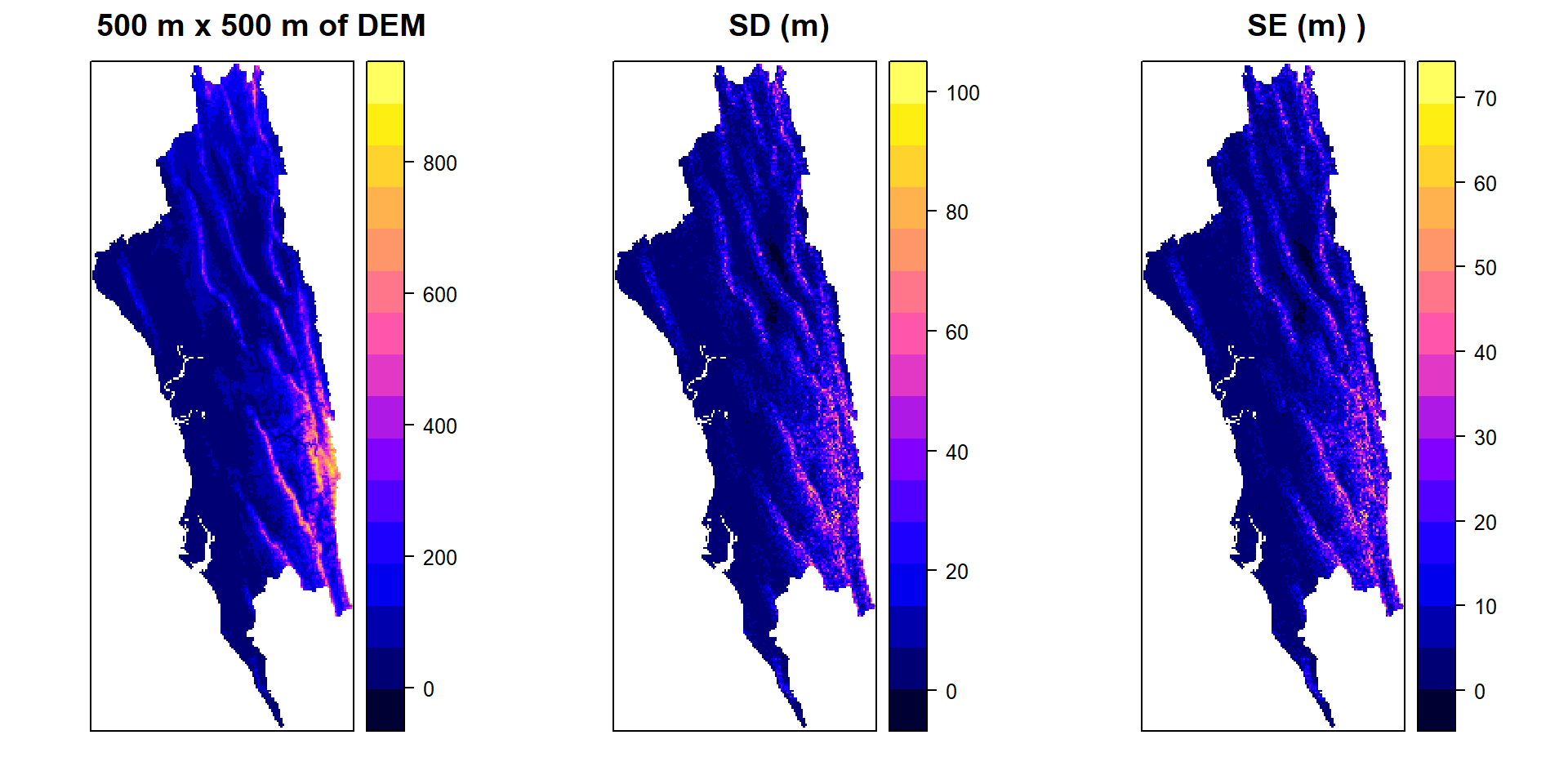

Disaggregation

If aggregating is the process of combining pixels, disaggregating is the process of splitting pixels into smaller ones. This operation is done with disagg(). Using the original 250m x 250m dem, each pixel will be disaggregated into smaller pixels (50 m x 50 m), once again using the fact argument.

Code

dem.50 <- disagg(dem.BTM, fact = 5)
dem.50

class       : SpatRaster 
dimensions  : 6645, 2605, 1  (nrow, ncol, nlyr)
resolution  : 50, 50  (x, y)
extent      : 648050.4, 778300.4, 295017.3, 627267.3  (xmin, xmax, ymin, ymax)
coord. ref. : +proj=tmerc +lat_0=0 +lon_0=90 +k=0.9996 +x_0=500000 +y_0=-2000000 +datum=WGS84 +units=m +no_defs 
source(s)   : memory
name        :     Band_1 
min value   :  -7.796429 
max value   : 985.049622

Code

spplot(dem.50, main="50 m x 50 m of DEM")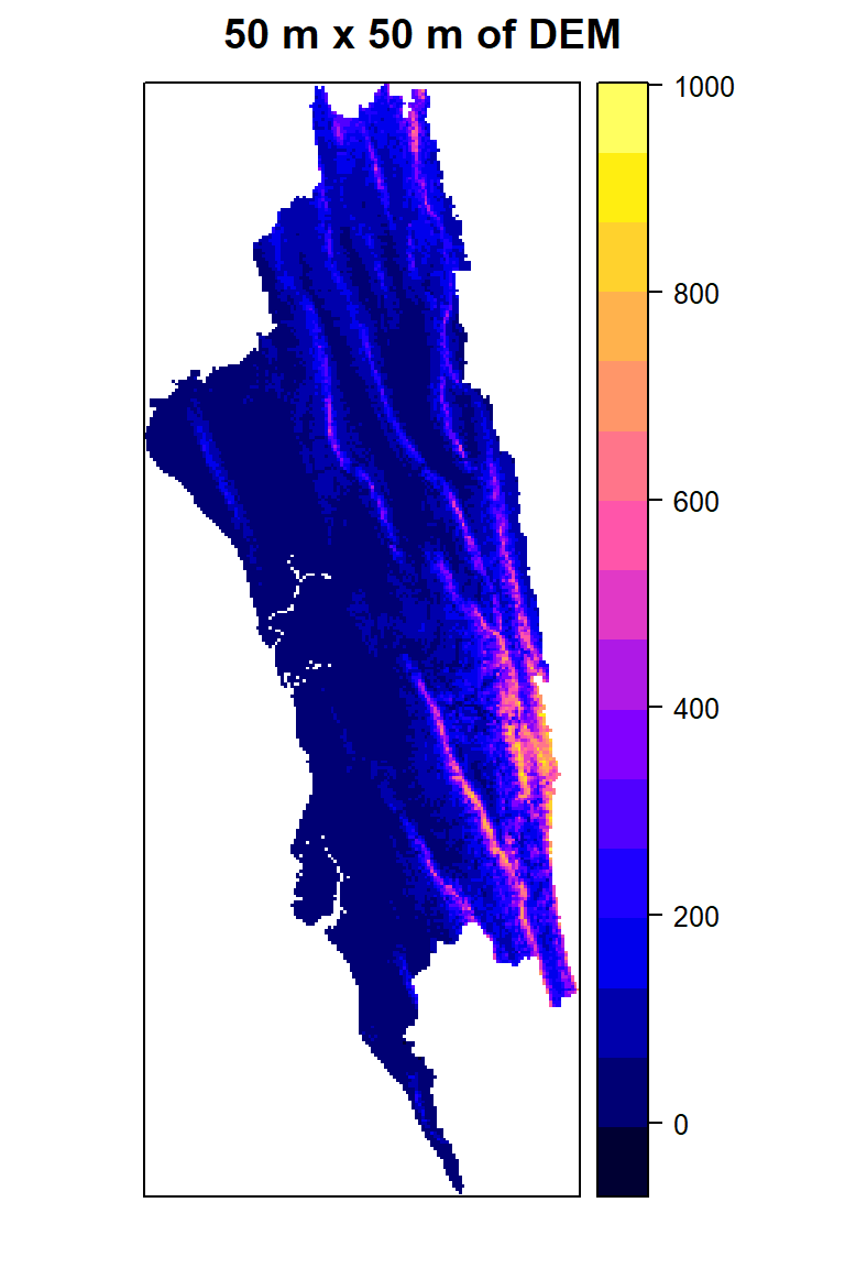

Resampling

Resampling is a technique used in geospatial analysis to change the spatial resolution or alignment of raster datasets. Resampling involves calculating new pixel values based on the original pixel values within a defined neighborhood or using interpolation methods. It’s often used when you need to match the resolution of one raster to another, change the resolution of a raster for analysis, or prepare data for visualization.

We will re-sample 500 m raster to 250 raster again using dem (250 m). We will use resample() function. Here two methods available: bilinear for bilinear interpolation, or **ngb* for using the nearest neighbor. First argument is a raster object to be re-sampled and second argument is raster object with parameters that first raster should be re-sampled to.

Code

dem.250m<-resample(mean.DEM, dem.BTM, method='bilinear') #
dem.250m

class       : SpatRaster 
dimensions  : 1329, 521, 1  (nrow, ncol, nlyr)
resolution  : 250, 250  (x, y)
extent      : 648050.4, 778300.4, 295017.3, 627267.3  (xmin, xmax, ymin, ymax)
coord. ref. : +proj=tmerc +lat_0=0 +lon_0=90 +k=0.9996 +x_0=500000 +y_0=-2000000 +datum=WGS84 +units=m +no_defs 
source(s)   : memory
name        :     Band_1 
min value   :  -3.292471 
max value   : 908.095215

Code

spplot(dem.250m, main="Resampled DEM - 250 m x 250 m")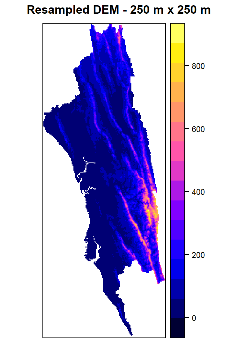

Mosaic

Raster mosaicking is the process of combining multiple raster datasets to create a single, continuous raster dataset that covers a larger geographic area. Mosaicking is commonly used when you have multiple raster images that need to be merged into a seamless and complete representation of a larger region. This technique is often employed in remote sensing, geospatial analysis, and cartography.

We will use merge() function to mosaic four raster in ./Raster/HILLY_DEM folder to create a seamless raster of hilly area of Bangladesh

Code

DEM.input <- list.files(path= paste0(dataFolder,".//Raster/HILLY_DEM"),pattern=".tiff$",full.names=T)   
DEM.input

[1] "G:\\My Drive\\Data\\Bangladesh\\.//Raster/HILLY_DEM/bandarban_dem_BTM.tiff"   
[2] "G:\\My Drive\\Data\\Bangladesh\\.//Raster/HILLY_DEM/chittagong_dem_BTM.tiff"  
[3] "G:\\My Drive\\Data\\Bangladesh\\.//Raster/HILLY_DEM/cox_bazar_dem_BTM.tiff"   
[4] "G:\\My Drive\\Data\\Bangladesh\\.//Raster/HILLY_DEM/khagrachhari_dem_BTM.tiff"
[5] "G:\\My Drive\\Data\\Bangladesh\\.//Raster/HILLY_DEM/rangamati_dem_BTM.tiff"

Code

r <- lapply(DEM.input, raster::raster)
r

[[1]]
class      : RasterLayer 
dimensions : 520, 261, 135720  (nrow, ncol, ncell)
resolution : 250, 250  (x, y)
extent     : 712800.4, 778050.4, 344017.3, 474017.3  (xmin, xmax, ymin, ymax)
crs        : +proj=tmerc +lat_0=0 +lon_0=90 +k=0.9996 +x_0=500000 +y_0=-2000000 +datum=WGS84 +units=m +no_defs 
source     : bandarban_dem_BTM.tiff 
names      : Band_1 
values     : -1.773466, 985.0496  (min, max)


[[2]]
class      : RasterLayer 
dimensions : 500, 323, 161500  (nrow, ncol, ncell)
resolution : 250, 250  (x, y)
extent     : 648050.4, 728800.4, 418267.3, 543267.3  (xmin, xmax, ymin, ymax)
crs        : +proj=tmerc +lat_0=0 +lon_0=90 +k=0.9996 +x_0=500000 +y_0=-2000000 +datum=WGS84 +units=m +no_defs 
source     : chittagong_dem_BTM.tiff 
names      : Band_1 
values     : -4.444613, 279.4592  (min, max)


[[3]]
class      : RasterLayer 
dimensions : 523, 219, 114537  (nrow, ncol, ncell)
resolution : 250, 250  (x, y)
extent     : 690300.4, 745050.4, 295017.3, 425767.3  (xmin, xmax, ymin, ymax)
crs        : +proj=tmerc +lat_0=0 +lon_0=90 +k=0.9996 +x_0=500000 +y_0=-2000000 +datum=WGS84 +units=m +no_defs 
source     : cox_bazar_dem_BTM.tiff 
names      : Band_1 
values     : -7.796429, 232.1743  (min, max)


[[4]]
class      : RasterLayer 
dimensions : 464, 191, 88624  (nrow, ncol, ncell)
resolution : 250, 250  (x, y)
extent     : 675550.4, 723300.4, 510267.3, 626267.3  (xmin, xmax, ymin, ymax)
crs        : +proj=tmerc +lat_0=0 +lon_0=90 +k=0.9996 +x_0=500000 +y_0=-2000000 +datum=WGS84 +units=m +no_defs 
source     : khagrachhari_dem_BTM.tiff 
names      : Band_1 
values     : 13.54026, 477.2253  (min, max)


[[5]]
class      : RasterLayer 
dimensions : 834, 298, 248532  (nrow, ncol, ncell)
resolution : 250, 250  (x, y)
extent     : 697800.4, 772300.4, 418767.3, 627267.3  (xmin, xmax, ymin, ymax)
crs        : +proj=tmerc +lat_0=0 +lon_0=90 +k=0.9996 +x_0=500000 +y_0=-2000000 +datum=WGS84 +units=m +no_defs 
source     : rangamati_dem_BTM.tiff 
names      : Band_1 
values     : 10.69665, 963.0776  (min, max)

Code

r1<-do.call(merge, c(r, tolerance = 1))

Code

spplot(r1, main="Mosaic DEM (m)")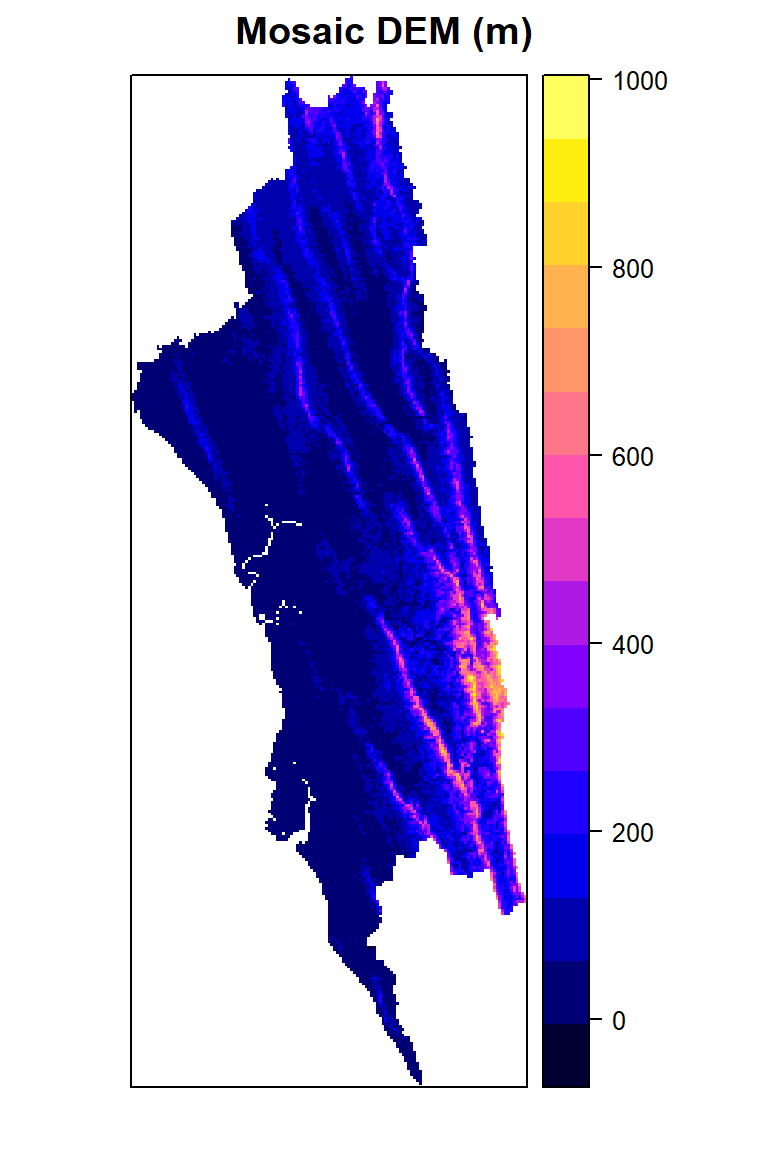

Raster to vector conversion

For convert raster data to spatial point data frame, we will use rasterToPoints() function and then we will apply as.data.frame() function to convert a regular data frame

Code

dataFolder<-"G:\\My Drive\\Data\\Bangladesh\\"
# if data in working directory
r<-raster(paste0(dataFolder, "/Raster/hilly_DEM_BTM.tiff"))

Code

SPDF <- rasterToPoints(r)
str(SPDF)

 num [1:310665, 1:3] 720925 720175 720425 720675 720925 ...
 - attr(*, "dimnames")=List of 2
  ..$ : NULL
  ..$ : chr [1:3] "x" "y" "Band_1"

Code

df<-as.data.frame(SPDF)
head(df)

         x        y   Band_1
1 720925.4 627142.3 357.0371
2 720175.4 626892.3 318.1637
3 720425.4 626892.3 320.6357
4 720675.4 626892.3 317.4960
5 720925.4 626892.3 355.9710
6 721175.4 626892.3 440.9489

Code

#write.csv(df, paste0(dataFolder,"GP_ElEV.csv", row.names = F))

Vector to raster conversion

Converting vector data to raster data is a common operation in geospatial analysis, allowing you to represent vector features as pixel values in a raster grid. This conversion is often done when you need to integrate vector data with other raster datasets, perform raster-based analysis, or prepare data for modeling or visualization. In R, you can perform vector to raster conversion using packages like raster and terra. Here’s how you can use these packages to convert vector data to raster data:

We will create raster of district wise boro production in Bangladesh. We will use raster::rasterize() function to create this raster similar resoluation of DEM (250 m x 25 m)

Code

dataFolder<-"G:\\My Drive\\Data\\Bangladesh\\"
# if data in working directory
poly<-raster::shapefile(paste0(dataFolder, "Shapefiles/bd_district_rice_production_2018_2019_BTM.shp")) 
bd.dem<-raster::raster(paste0(dataFolder, "Raster/DEM.tif"))

Code

poly$Boro_1000<-poly$Boro/1000

Code

# Define the extent, resolution, and target raster template
r <- raster::raster(bd.dem)
extent(r) <- raster::extent(poly)
rp <- raster::rasterize(poly, r, 'Boro_1000')
rp

class      : RasterLayer 
dimensions : 2680, 1919, 5142920  (nrow, ncol, ncell)
resolution : 249.9291, 249.3885  (x, y)
extent     : 298487.8, 778101.8, 278578.1, 946939.2  (xmin, xmax, ymin, ymax)
crs        : +proj=tmerc +lat_0=0 +lon_0=90 +k=0.9996 +x_0=500000 +y_0=0 +datum=WGS84 +units=m +no_defs 
source     : memory
names      : layer 
values     : 0, 1018.506  (min, max)

Code

spplot(rp, main = "Boro Production Raster (MT X 1000)")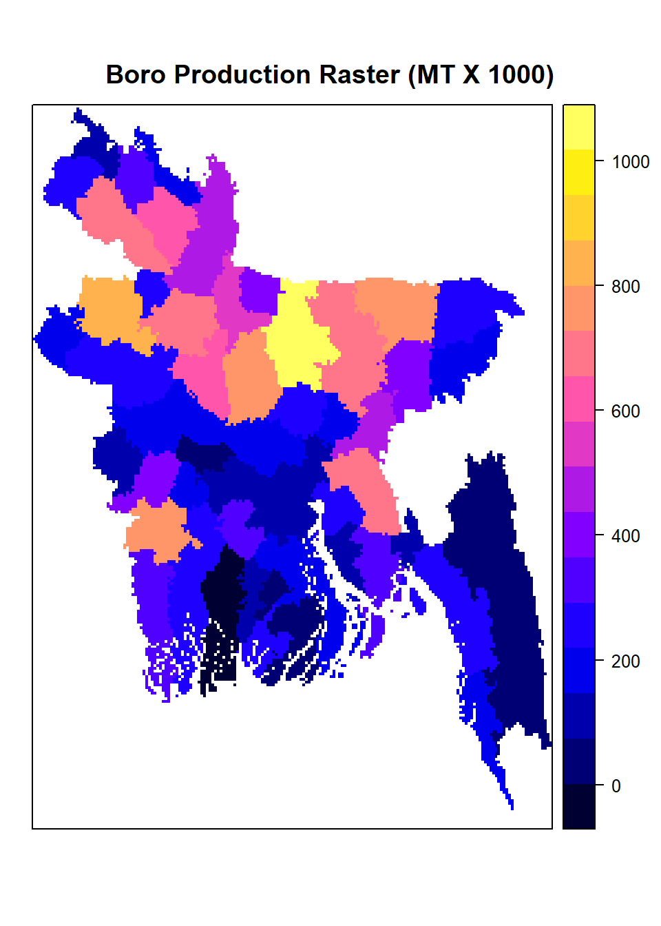

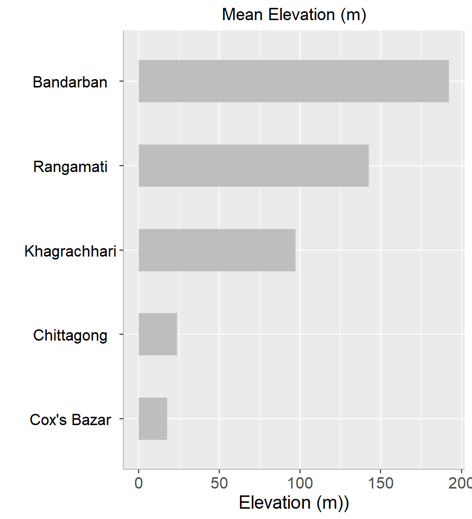
Zoal Statistics

Zonal statistics is a geospatial analysis technique that involves calculating summary statistics within predefined zones or regions of interest. These regions are typically defined by a vector dataset, such as polygons representing administrative boundaries, land parcels, or any other spatial units. Zonal statistics allow you to extract information from raster datasets based on the spatial boundaries defined by the vector features.

In this exercise we will calculate mean elevation five district of hilly area of Bangladesh.

Code

dataFolder<-"G:\\My Drive\\Data\\Bangladesh\\"
# if data in working directory
hilly.dist<-raster::shapefile(paste0(dataFolder, "Shapefiles/hilly_district_BTM.shp"))
hilly.dem<-raster::raster(paste0(dataFolder, "Raster/hilly_dem_BTM.tiff"))

We can apply raster::extract() function to calculate any statistics by zones

Code

mean.elevation <- extract(hilly.dem, hilly.dist, fun=mean, na.rm=TRUE, df=TRUE)
mean.elevation

  ID    Band_1
1  1 192.32852
2  2  23.79157
3  3  17.54851
4  4  97.13356
5  5 142.51197

Code

# add district name
mean.elevation$dist.name<-levels(as.factor(hilly.dist$ADM2_EN))
mean.elevation

  ID    Band_1    dist.name
1  1 192.32852    Bandarban
2  2  23.79157   Chittagong
3  3  17.54851  Cox's Bazar
4  4  97.13356 Khagrachhari
5  5 142.51197    Rangamati

You can visualize the mean elevation using ggplot():

Code

ggplot(as.data.frame(mean.elevation), aes(x=reorder(dist.name, +Band_1), y=Band_1)) + 
  geom_bar(stat="identity", position=position_dodge(),width=0.5, fill="gray") +
  # add y-axis title and x-axis title leave blank
  labs(y="Elevation (m))", x = "")+ 
  # add plot title
  ggtitle("Mean Elevation (m)")+
  coord_flip()+
  # customize plot themes
  theme(
        axis.line = element_line(colour = "gray"),
        # plot title position at center
        plot.title = element_text(hjust = 0.5),
        # axis title font size
        axis.title.x = element_text(size = 14), 
        # X and  axis font size
        axis.text.y=element_text(size=12,vjust = 0.5, hjust=0.5, colour='black'),
        axis.text.x = element_text(size=12))

Working with Raster Data in R

Load R packages

Data

Basic Raster Operation

Check projection system

Check raster attribute

Raster extent

Raster statistics

Histogram of raster

Plot raster

Clipping

Reclassification

Histogram

Quantile

Focal Statistics

Raster Algebra

Aggregation

Disaggregation

Resampling

Mosaic

Raster to vector conversion

Vector to raster conversion

Zoal Statistics

Further Reading