H2O’s Deep Learning is based on a multi-layer feedforward artificial neural network that is trained with stochastic gradient descent using back-propagation. The network can contain a large number of hidden layers consisting of neurons with tanh, rectifier, and maxout activation functions. Advanced features such as adaptive learning rate, rate annealing, momentum training, dropout, L1 or L2 regularization, checkpointing, and grid search enable high predictive accuracy. Each compute node trains a copy of the global model parameters on its local data with multi-threading (asynchronously) and contributes periodically to the global model via model averaging across the network.
Data
In this exercise we will use following synthetic data set and use DEM, Slope, TPI, MAT, MAP, NDVI, NLCD, FRG to fit Deep Neural Network regression model. This data was created with AI using gp_soil_data data set
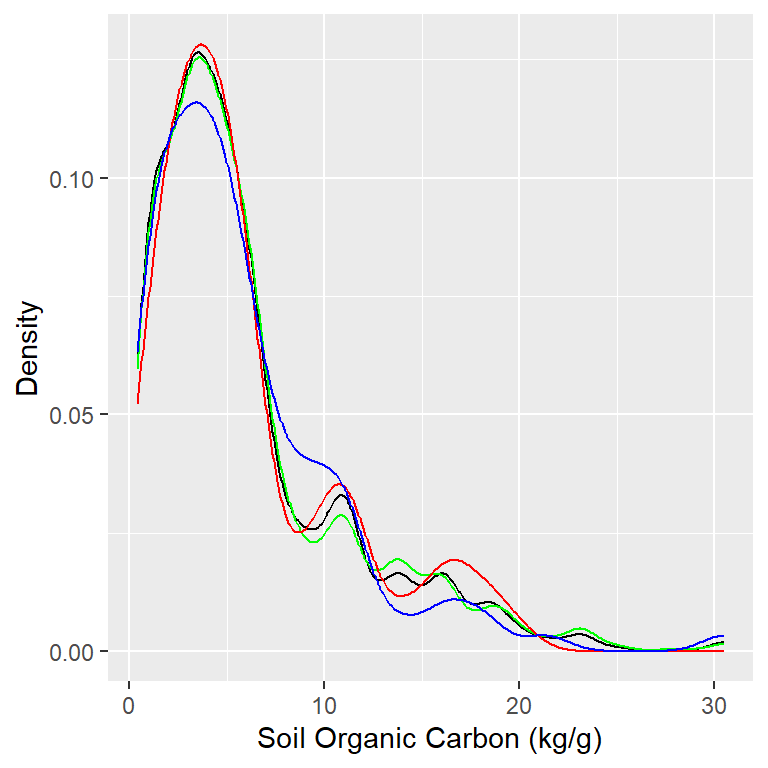
The data set (n = 1408) will randomly split into sub-sets for training (70%), validation (15%) and test data (15%). The validation data will be used to optimized the model parameters during the tuning and training processes. The test data set will be used as the hold-out data to evaluate the DNN model.
Code
library(tidymodels)set.seed(1245) # for reproducibilitysplit_01 <-initial_split(df, prop =0.7, strata = SOC)train <- split_01 %>%training()test_valid <- split_01 %>%testing()split_02 <-initial_split(test_valid, prop =0.5, strata = SOC)test <- split_02 %>%training()valid <- split_02 %>%testing()# Density plot all, train and test data ggplot()+geom_density(data = df, aes(SOC))+geom_density(data = train, aes(SOC), color ="green")+geom_density(data = test, aes(SOC), color ="red") +geom_density(data = valid, aes(SOC), color ="blue") +xlab("Soil Organic Carbon (kg/g)") +ylab("Density")
H2O is not running yet, starting it now...

Note:  In case of errors look at the following log files:
    C:\Users\zahmed2\AppData\Local\Temp\1\RtmpMf4ipQ\file6dec254463ef/h2o_zahmed2_started_from_r.out
    C:\Users\zahmed2\AppData\Local\Temp\1\RtmpMf4ipQ\file6dec169a6288/h2o_zahmed2_started_from_r.err


Starting H2O JVM and connecting:  Connection successful!

R is connected to the H2O cluster:
    H2O cluster uptime:         3 seconds 218 milliseconds
    H2O cluster timezone:       America/New_York
    H2O data parsing timezone:  UTC
    H2O cluster version:        3.40.0.4
    H2O cluster version age:    3 months and 23 days
    H2O cluster name:           H2O_started_from_R_zahmed2_frf170
    H2O cluster total nodes:    1
    H2O cluster total memory:   148.00 GB
    H2O cluster total cores:    40
    H2O cluster allowed cores:  40
    H2O cluster healthy:        TRUE
    H2O Connection ip:          localhost
    H2O Connection port:        54321
    H2O Connection proxy:       NA
    H2O Internal Security:      FALSE
    R Version:                  R version 4.3.1 (2023-06-16 ucrt)
Code
#disable progress bar for RMarkdownh2o.no_progress() # Optional: remove anything from previous sessionh2o.removeAll()
standardize: logical. If enabled, automatically standardize the data.
distribution:
activation: Specify the activation function. One of:
tanh
tanh_with_dropout
rectifier (default)
rectifier_with_dropout
maxout (not supported when autoencoder is enabled)
maxout_with_dropout
hidden: Specify the hidden layer sizes (e.g., (100,100)). The value must be positive. This option defaults to (200,200).
adaptive_rate: Specify whether to enable the adaptive learning rate (ADADELTA). This option defaults to True (enabled).
epochs: Specify the number of times to iterate (stream) the dataset. The value can be a fraction. This option defaults to 10.
epsilon: (Applicable only if adaptive_rate=True) Specify the adaptive learning rate time smoothing factor to avoid dividing by zero. This option defaults to 1e-08.
input_dropout_ratio: Specify the input layer dropout ratio to improve generalization. Suggested values are 0.1 or 0.2. This option defaults to 0.
l1: Specify the L1 regularization to add stability and improve generalization; sets the value of many weights to 0 (default).
l2: Specify the L2 regularization to add stability and improve generalization; sets the value of many weights to smaller values. Defaults to 0.
max_w2: Specify the constraint for the squared sum of the incoming weights per unit (e.g. for rectifier). Defaults to 3.4028235e+38.
momentum_start: (Applicable only if adaptive_rate=False) Specify the initial momentum at the beginning of training; we suggest 0.5. This option defaults to 0.
rate: (Applicable only if adaptive_rate=False) Specify the learning rate. Higher values result in a less stable model, while lower values lead to slower convergence. This option defaults to 0.005.
rate_annealing: Learning rate decay, (Applicable only if adaptive_rate=False) Specify the rate annealing value. rate(1+ rate_annealing × samples), This option defaults to 1e-06.
rate_decay: (Applicable only if adaptive_rate=False) Specify the rate decay factor between layers. N-th layer: rate × rate_decay(n−1). This options defaults to 1.
regression_stop: (Regression models only) Specify the stopping criterion for regression error (MSE) on the training data. When the error is at or below this threshold, training stops. To disable this option, enter -1. This option defaults to 1e-06.
rho: (Applicable only if adaptive_rate is enabled) Specify the adaptive learning rate time decay factor. This option defaults to 0.99.
shuffle_training_data: Specify whether to shuffle the training data. This option is recommended if the training data is replicated and the value of train_samples_per_iteration is close to the number of nodes times the number of rows. This option defaults to False (disabled).
stopping_tolerance = Relative tolerance for metric-based stopping criterion
stopping_rounds = Early stopping based on convergence of stopping_metric.Defaults to 5.
stopping_metric = Metric to use for early stopping
variable_importances: Specify whether to compute variable importance. This option defaults to True (enabled).
H2ORegressionMetrics: deeplearning
** Reported on cross-validation data. **
** 5-fold cross-validation on training data (Metrics computed for combined holdout predictions) **

MSE:  10.94951
RMSE:  3.309005
MAE:  2.208836
RMSLE:  NaN
Mean Residual Deviance :  10.94951
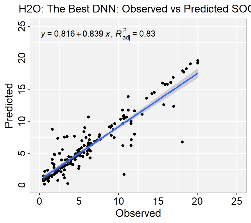
Fit the Best DNN model with hyperparameter tunning
H2O Grid Search is a hyperparameter optimization technique used in the H2O machine learning framework. It involves a systematic search through a specified subset of hyperparameters of a machine learning model to find the optimal combination of hyperparameters that maximizes the performance metric of interest, such as RMSE or AUC.
H2O supports two types of grid search – traditional (or “cartesian”) grid search and random grid search. In a cartesian grid search, users specify a set of values for each hyperparameter that they want to search over, and H2O will train a model for every combination of the hyperparameter values. This means that if you have three hyperparameters and you specify 5, 10 and 2 values for each, your grid will contain a total of 5102 = 100 models.
Data
In this exercise we will use following synthetic data set and use DEM, Slope, TPI, MAT, MAP,NDVI, NLCD, FRG to fit Deep Neural Network regression model. This data was created with AI using gp_soil_data data set
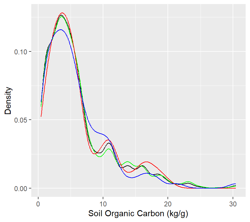
The data set (n = 1408) will randomly split into sub-sets for training (70%), validation (15%) and test data (15%). The validation data will be used to optimized the model parameters during the tuning and training processes. The test data set will be used as the hold-out data to evaluate the DNN model.
Code
library(tidymodels)set.seed(1245) # for reproducibilitysplit_01 <-initial_split(df, prop =0.7, strata = SOC)train <- split_01 %>%training()test_valid <- split_01 %>%testing()split_02 <-initial_split(test_valid, prop =0.5, strata = SOC)test <- split_02 %>%training()valid <- split_02 %>%testing()# Density plot all, train and test data ggplot()+geom_density(data = df, aes(SOC))+geom_density(data = train, aes(SOC), color ="green")+geom_density(data = test, aes(SOC), color ="red") +geom_density(data = valid, aes(SOC), color ="blue") +xlab("Soil Organic Carbon (kg/g)") +ylab("Density")
H2O Grid Search is a hyperparameter optimization technique used in the H2O machine learning framework. It involves a systematic search through a specified subset of hyperparameters of a machine learning model to find the optimal combination of hyperparameters that maximizes the performance metric of interest, such as RMSE or AUC.
In a grid search, a set of hyperparameters is defined, and a range of values is specified for each hyperparameter. The grid search algorithm then systematically evaluates all possible combinations of hyperparameter values, training and evaluating a model for each combination, and selecting the combination that performs the best on the validation set.
H2O supports two types of grid search – traditional (or “cartesian”) grid search and random grid search. In a cartesian grid search, users specify a set of values for each hyperparameter that they want to search over, and H2O will train a model for every combination of the hyperparameter values. This means that if you have three hyperparameters and you specify 5, 10 and 2 values for each, your grid will contain a total of 5102 = 100 models.
# Get Model IDDNN_get_grid <-h2o.getGrid("DNN_grid_IDs",sort_by="RMSE",decreasing=F)# Get the best RF modelbest_DNN <-h2o.getModel(DNN_get_grid@model_ids[[1]])best_DNN
Model Details:
==============

H2ORegressionModel: deeplearning
Model ID:  DNN_grid_IDs_model_5
Status of Neuron Layers: predicting SOC, regression, gaussian distribution, Quadratic loss, 22,201 weights/biases, 268.9 KB, 501,330 training samples, mini-batch size 1
  layer units   type dropout       l1       l2 mean_rate rate_rms momentum
1     1    18  Input  0.01 %       NA       NA        NA       NA       NA
2     2   100   Tanh  0.00 % 0.000000 0.000010  0.142395 0.304260 0.000000
3     3   100   Tanh  0.00 % 0.000000 0.000010  0.208295 0.103840 0.000000
4     4   100   Tanh  0.00 % 0.000000 0.000010  0.442853 0.368074 0.000000
5     5     1 Linear      NA 0.000000 0.000010  0.010988 0.007448 0.000000
  mean_weight weight_rms mean_bias bias_rms
1          NA         NA        NA       NA
2   -0.002011   0.261768 -0.025849 0.158819
3   -0.000508   0.210741 -0.039715 0.402734
4   -0.001515   0.188434 -0.009917 0.207660
5   -0.006977   0.139361  0.194065 0.000000


H2ORegressionMetrics: deeplearning
** Reported on training data. **
** Metrics reported on full training frame **

MSE:  0.1709891
RMSE:  0.4135083
MAE:  0.2467445
RMSLE:  0.1020061
Mean Residual Deviance :  0.1709891


H2ORegressionMetrics: deeplearning
** Reported on validation data. **
** Metrics reported on full validation frame **

MSE:  3.484517
RMSE:  1.866686
MAE:  0.9583159
RMSLE:  0.2979063
Mean Residual Deviance :  3.484517


H2ORegressionMetrics: deeplearning
** Reported on cross-validation data. **
** 5-fold cross-validation on training data (Metrics computed for combined holdout predictions) **

MSE:  8.65523
RMSE:  2.941977
MAE:  1.728109
RMSLE:  0.4379155
Mean Residual Deviance :  8.65523


Cross-Validation Metrics Summary:
                           mean       sd cv_1_valid cv_2_valid cv_3_valid
mae                    1.726087 0.324924   1.531918   1.557160   2.236158
mean_residual_deviance 8.652568 2.681121   6.440247   8.918200  11.117817
mse                    8.652568 2.681121   6.440247   8.918200  11.117817
r2                     0.665135 0.105993   0.712035   0.667448   0.595563
residual_deviance      8.652568 2.681121   6.440247   8.918200  11.117817
rmse                   2.911709 0.467064   2.537764   2.986336   3.334339
rmsle                  0.433899 0.064433   0.381605   0.438783   0.517207
                       cv_4_valid cv_5_valid
mae                      1.446334   1.858864
mean_residual_deviance   5.428764  11.357812
mse                      5.428764  11.357812
r2                       0.812584   0.538046
residual_deviance        5.428764  11.357812
rmse                     2.329971   3.370135
rmsle                    0.359990   0.471913
Model performance
Code
# training performanceh2o.performance(best_DNN, h_train)
Model explainability refers to the ability to understand and interpret the decisions made by a machine learning model. In other words, it is the ability to explain how a model arrives at its predictions or classifications.
Explainability is particularly important in applications where decisions made by the model have significant real-world consequences, such as in healthcare, finance, and legal fields. It is also important for regulatory compliance, where models must be auditable and transparent.
The h2o.explain() function generates a list of explanations – individual units of explanation such as a Partial Dependence plot or a Variable Importance plot. Most of the explanations are visual – these plots can also be created by individual utility functions outside the h2o.explain() function.
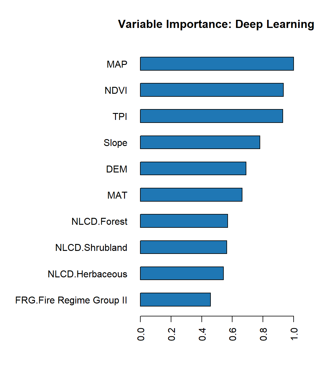
Retrieve the variable importance.
Code
h2o.varimp(best_DNN)
Variable Importances:
                    variable relative_importance scaled_importance percentage
1                        MAP            1.000000          1.000000   0.107677
2                       NDVI            0.932508          0.932508   0.100410
3                        TPI            0.930439          0.930439   0.100187
4                      Slope            0.779952          0.779952   0.083983
5                        DEM            0.688935          0.688935   0.074183
6                        MAT            0.663888          0.663888   0.071486
7                NLCD.Forest            0.569794          0.569794   0.061354
8             NLCD.Shrubland            0.563952          0.563952   0.060725
9            NLCD.Herbaceous            0.541844          0.541844   0.058344
10  FRG.Fire Regime Group II            0.456929          0.456929   0.049201
11 FRG.Fire Regime Group III            0.427719          0.427719   0.046056
12   NLCD.Planted/Cultivated            0.377079          0.377079   0.040603
13  FRG.Fire Regime Group IV            0.363503          0.363503   0.039141
14   FRG.Fire Regime Group I            0.352672          0.352672   0.037975
15   FRG.Fire Regime Group V            0.330626          0.330626   0.035601
16     FRG.Indeterminate FRG            0.307173          0.307173   0.033076
17           FRG.missing(NA)            0.000000          0.000000   0.000000
18          NLCD.missing(NA)            0.000000          0.000000   0.000000
Variable Importance Plot
Code
h2o.varimp_plot(best_DNN)
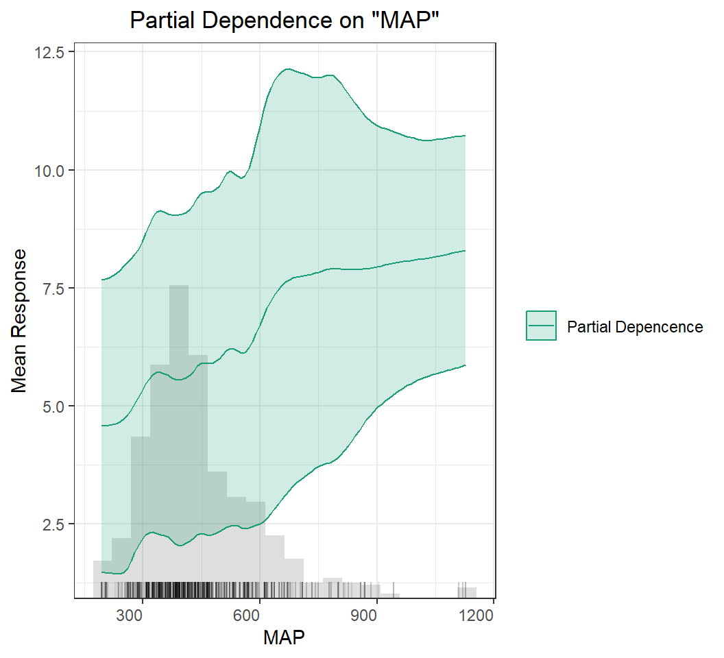
Partial Dependence (PD) Plots
A partial dependence plot (PDP) is a graphical tool for understanding the relationship between a particular input feature and the output of a machine learning model.
A PDP shows the marginal effect of a single feature on the predicted outcome while holding all other features at a fixed value or their average value. The PDP can help to visualize the shape and direction of the relationship between the feature and the output, and can also help to identify any non-linearities or interactions between the feature and other features in the model.
To create a PDP, the value of the feature of interest is varied over its range, and the model’s predicted output is recorded for each value. The resulting data is then plotted on a graph, with the feature’s value on the x-axis and the predicted output on the y-axis.
PDPs can be used to gain insights into how a model is making its predictions and to identify which features are most important for the model’s output. They can also be used to identify potential biases in the model or to detect interactions between features that may be difficult to detect using other methods.
Code
h2o.pd_multi_plot(best_DNN, h_train, "MAP")
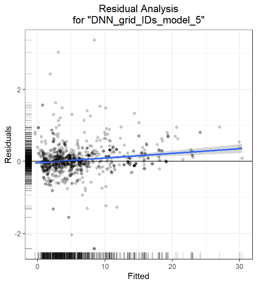
Residual Analysis
Residual Analysis plots the fitted values vs residuals on a test dataset. Ideally, residuals should be randomly distributed. Patterns in this plot can indicate potential problems with the model selection, e.g., using simpler model than necessary, not accounting for heteroscedasticity, autocorrelation, etc. Note that if you see “striped” lines of residuals, that is an artifact of having an integer valued (vs a real valued) response variable
# Deep Neural Network with h20 {.unnumbered}H2O’s Deep Learning is based on a multi-layer feedforward artificial neural network that is trained with stochastic gradient descent using back-propagation. The network can contain a large number of hidden layers consisting of neurons with tanh, rectifier, and maxout activation functions. Advanced features such as adaptive learning rate, rate annealing, momentum training, dropout, L1 or L2 regularization, checkpointing, and grid search enable high predictive accuracy. Each compute node trains a copy of the global model parameters on its local data with multi-threading (asynchronously) and contributes periodically to the global model via model averaging across the network.#### DataIn this exercise we will use following synthetic data set and use DEM, Slope, TPI, MAT, MAP, NDVI, NLCD, FRG to fit Deep Neural Network regression model. This data was created with AI using gp_soil_data data set [gp_soil_data_syn.csv](https://www.dropbox.com/s/c63etg7u5qql2y8/gp_soil_data_syn.csv?dl=0)```{r}#| warning: false#| error: false#| fig.width: 5#| fig.height: 4library(tidyverse)# define data folderdataFolder<-"E:/Dropbox/GitHub/Data/USA/"# Load datamf<-read_csv(paste0(dataFolder, "gp_soil_data_syn.csv"))# Create a data-framedf<-mf %>% dplyr::select(SOC, DEM, Slope, TPI, MAT, MAP,NDVI, NLCD, FRG)%>%glimpse()```#### Convert to factor```{r}#| warning: false#| error: falsedf$NLCD <-as.factor(df$NLCD)df$FRG <-as.factor(df$FRG)```#### Data splitThe data set (n = 1408) will randomly split into sub-sets for training (70%), validation (15%) and test data (15%). The validation data will be used to optimized the model parameters during the tuning and training processes. The test data set will be used as the hold-out data to evaluate the DNN model. ```{r}#| warning: false#| error: false#| fig.width: 4#| fig.height: 4library(tidymodels)set.seed(1245) # for reproducibilitysplit_01 <-initial_split(df, prop =0.7, strata = SOC)train <- split_01 %>%training()test_valid <- split_01 %>%testing()split_02 <-initial_split(test_valid, prop =0.5, strata = SOC)test <- split_02 %>%training()valid <- split_02 %>%testing()# Density plot all, train and test data ggplot()+geom_density(data = df, aes(SOC))+geom_density(data = train, aes(SOC), color ="green")+geom_density(data = test, aes(SOC), color ="red") +geom_density(data = valid, aes(SOC), color ="blue") +xlab("Soil Organic Carbon (kg/g)") +ylab("Density")```#### Import h2o```{r}#| warning: false#| error: falselibrary(h2o)h2o.init(nthreads =-1, max_mem_size ="148g", enable_assertions =FALSE) #disable progress bar for RMarkdownh2o.no_progress() # Optional: remove anything from previous sessionh2o.removeAll() ```#### Import data to h2o cluster```{r}#| warning: false#| error: falseh_df=as.h2o(df)h_train =as.h2o(train)h_test =as.h2o(test)h_valid =as.h2o(valid)``````{r}CV.xy<-as.data.frame(h_train)test.xy<-as.data.frame(h_test)```#### Define response and predictors```{r}#| warning: false#| error: falsey <-"SOC"x <-setdiff(names(h_df), y)```### Fit DNN model with few fixed prametersFirst we fit DNN model with following parameters:standardize: logical. If enabled, automatically standardize the data.distribution: activation: Specify the activation function. One of: - tanh - tanh_with_dropout - rectifier (default) - rectifier_with_dropout - maxout (not supported when autoencoder is enabled) - maxout_with_dropouthidden: Specify the hidden layer sizes (e.g., (100,100)). The value must be positive. This option defaults to (200,200).adaptive_rate: Specify whether to enable the adaptive learning rate (ADADELTA). This option defaults to True (enabled).epochs: Specify the number of times to iterate (stream) the dataset. The value can be a fraction. This option defaults to 10.epsilon: (Applicable only if adaptive_rate=True) Specify the adaptive learning rate time smoothing factor to avoid dividing by zero. This option defaults to 1e-08.input_dropout_ratio: Specify the input layer dropout ratio to improve generalization. Suggested values are 0.1 or 0.2. This option defaults to 0.l1: Specify the L1 regularization to add stability and improve generalization; sets the value of many weights to 0 (default).l2: Specify the L2 regularization to add stability and improve generalization; sets the value of many weights to smaller values. Defaults to 0.max_w2: Specify the constraint for the squared sum of the incoming weights per unit (e.g. for rectifier). Defaults to 3.4028235e+38.momentum_start: (Applicable only if adaptive_rate=False) Specify the initial momentum at the beginning of training; we suggest 0.5. This option defaults to 0.rate: (Applicable only if adaptive_rate=False) Specify the learning rate. Higher values result in a less stable model, while lower values lead to slower convergence. This option defaults to 0.005.rate_annealing: Learning rate decay, (Applicable only if adaptive_rate=False) Specify the rate annealing value. rate(1+ rate_annealing × samples), This option defaults to 1e-06.rate_decay: (Applicable only if adaptive_rate=False) Specify the rate decay factor between layers. N-th layer: rate × rate_decay(n−1). This options defaults to 1.regression_stop: (Regression models only) Specify the stopping criterion for regression error (MSE) on the training data. When the error is at or below this threshold, training stops. To disable this option, enter -1. This option defaults to 1e-06.rho: (Applicable only if adaptive_rate is enabled) Specify the adaptive learning rate time decay factor. This option defaults to 0.99.shuffle_training_data: Specify whether to shuffle the training data. This option is recommended if the training data is replicated and the value of train_samples_per_iteration is close to the number of nodes times the number of rows. This option defaults to False (disabled).stopping_tolerance = Relative tolerance for metric-based stopping criterionstopping_rounds = Early stopping based on convergence of stopping_metric.Defaults to 5.stopping_metric = Metric to use for early stoppingvariable_importances: Specify whether to compute variable importance. This option defaults to True (enabled).```{r}#| warning: false#| error: falseDNN <-h2o.deeplearning(model_id="DNN_model_ID", training_frame=h_train, validation_frame=h_valid, x=x, y=y, distribution ="AUTO",standardize =TRUE,shuffle_training_data =TRUE,activation ="tanh", hidden =c(100, 100, 100),epochs =500,adaptive_rate =TRUE, rate =0.005,rate_annealing =1e-06,rate_decay =1, rho =0.99,epsilon =1e-08,momentum_start =0.5,momentum_stable =0.99,input_dropout_ratio =0.0001,regression_stop =1e-06, l1 =0.0001, l2 =0.0001,max_w2 =3.4028235e+38,stopping_tolerance =0.001,stopping_rounds =3,stopping_metric ="RMSE", nfolds =5,keep_cross_validation_models =TRUE,keep_cross_validation_predictions =TRUE,variable_importances =TRUE,seed=1256 ) ```#### Scoring History```{r}#| warning: false#| error: false#| fig.width: 5#| fig.height: 4plot(DNN)```#### Model performance##### Training```{r}h2o.performance(DNN, h_train)```##### Cross-validation```{r}h2o.performance(DNN, xval=TRUE)```##### Validation data```{r}h2o.performance(DNN, h_valid)```##### Test data```{r}h2o.performance(DNN, h_test)```#### Prediction```{r message=FALSE, warning=FALSE}# test - predictiontest.pred.DNN<-as.data.frame(h2o.predict(object = DNN, newdata = h_test))test.xy$DNN_SOC<-test.pred.DNN$predict```We can plot observed and predicted values with fitted regression line with ggplot2```{r}#| warning: false#| error: false#| fig.width: 5.5#| fig.height: 4.5library(ggpmisc)formula<-y~xggplot(test.xy, aes(SOC,DNN_SOC)) +geom_point() +geom_smooth(method ="lm")+stat_poly_eq(use_label(c("eq", "adj.R2")), formula = formula) +ggtitle("H2O-DNN: Observed vs Predicted SOC ") +xlab("Observed") +ylab("Predicted") +scale_x_continuous(limits=c(0,22), breaks=seq(0, 22, 4))+scale_y_continuous(limits=c(0,22), breaks=seq(0, 22, 4)) +# Flip the barstheme(panel.background =element_rect(fill ="grey95",colour ="gray75",size =0.5, linetype ="solid"),axis.line =element_line(colour ="grey"),plot.title =element_text(size =14, hjust =0.5),axis.title.x =element_text(size =14),axis.title.y =element_text(size =14),axis.text.x=element_text(size=13, colour="black"),axis.text.y=element_text(size=13,angle =90,vjust =0.5, hjust=0.5, colour='black'))``````{r}# remove all objectrm(list =ls())```### Fit the Best DNN model with hyperparameter tunningH2O Grid Search is a hyperparameter optimization technique used in the H2O machine learning framework. It involves a systematic search through a specified subset of hyperparameters of a machine learning model to find the optimal combination of hyperparameters that maximizes the performance metric of interest, such as RMSE or AUC.H2O supports two types of grid search -- traditional (or "cartesian") grid search and random grid search. In a cartesian grid search, users specify a set of values for each hyperparameter that they want to search over, and H2O will train a model for every combination of the hyperparameter values. This means that if you have three hyperparameters and you specify 5, 10 and 2 values for each, your grid will contain a total of 5*10*2 = 100 models.#### DataIn this exercise we will use following synthetic data set and use DEM, Slope, TPI, MAT, MAP,NDVI, NLCD, FRG to fit Deep Neural Network regression model. This data was created with AI using gp_soil_data data set [gp_soil_data_syn.csv](https://www.dropbox.com/s/c63etg7u5qql2y8/gp_soil_data_syn.csv?dl=0)```{r}#| warning: false#| error: false#| fig.width: 5#| fig.height: 4library(tidyverse)# define data folderdataFolder<-"E:/Dropbox/GitHub/Data/USA/"# Load datamf<-read_csv(paste0(dataFolder, "gp_soil_data_syn.csv"))# Create a data-framedf<-mf %>% dplyr::select(SOC, DEM, Slope, TPI, MAT, MAP,NDVI, NLCD, FRG)```#### Convert to factor```{r}#| warning: false#| error: falsedf$NLCD <-as.factor(df$NLCD)df$FRG <-as.factor(df$FRG)```#### Data splitThe data set (n = 1408) will randomly split into sub-sets for training (70%), validation (15%) and test data (15%). The validation data will be used to optimized the model parameters during the tuning and training processes. The test data set will be used as the hold-out data to evaluate the DNN model. ```{r}#| warning: false#| error: false#| fig.width: 4.5#| fig.height: 4library(tidymodels)set.seed(1245) # for reproducibilitysplit_01 <-initial_split(df, prop =0.7, strata = SOC)train <- split_01 %>%training()test_valid <- split_01 %>%testing()split_02 <-initial_split(test_valid, prop =0.5, strata = SOC)test <- split_02 %>%training()valid <- split_02 %>%testing()# Density plot all, train and test data ggplot()+geom_density(data = df, aes(SOC))+geom_density(data = train, aes(SOC), color ="green")+geom_density(data = test, aes(SOC), color ="red") +geom_density(data = valid, aes(SOC), color ="blue") +xlab("Soil Organic Carbon (kg/g)") +ylab("Density")```#### Import h2o```{r}#| warning: false#| error: falselibrary(h2o)h2o.init(nthreads =-1, max_mem_size ="148g", enable_assertions =FALSE) #disable progress bar for RMarkdownh2o.no_progress() # Optional: remove anything from previous sessionh2o.removeAll() ```#### Import data to h2o cluster```{r}#| warning: false#| error: falseh_df=as.h2o(df)h_train =as.h2o(train)h_test =as.h2o(test)h_valid =as.h2o(valid)``````{r}CV.xy<-as.data.frame(h_train)test.xy<-as.data.frame(h_test)```#### Define response and predictors```{r}#| warning: false#| error: falsey <-"SOC"x <-setdiff(names(h_df), y)```#### Fit DNN model with hyperparameter tunningH2O Grid Search is a hyperparameter optimization technique used in the H2O machine learning framework. It involves a systematic search through a specified subset of hyperparameters of a machine learning model to find the optimal combination of hyperparameters that maximizes the performance metric of interest, such as RMSE or AUC.In a grid search, a set of hyperparameters is defined, and a range of values is specified for each hyperparameter. The grid search algorithm then systematically evaluates all possible combinations of hyperparameter values, training and evaluating a model for each combination, and selecting the combination that performs the best on the validation set.H2O supports two types of grid search -- traditional (or "cartesian") grid search and random grid search. In a cartesian grid search, users specify a set of values for each hyperparameter that they want to search over, and H2O will train a model for every combination of the hyperparameter values. This means that if you have three hyperparameters and you specify 5, 10 and 2 values for each, your grid will contain a total of 5*10*2 = 100 models.#### Define DNN Hyper-parameters```{r}#| warning: false#| error: falseDNN_hyper_params <-list(activation =c("Rectifier", "Maxout", "Tanh", "RectifierWithDropout", "MaxoutWithDropout","TanhWithDropout"),hidden =list( c(50, 50, 50, 50), c(100, 100, 100), c(200, 200, 200)),epochs =c(50, 100, 200, 500),l1 =c(0, 0.00001, 0.0001), l2 =c(0, 0.00001, 0.0001),rate =c(0, 01, 0.005, 0.001),rate_decay =c(0.5, 1.0, 1.5),rate_annealing =c(1e-5, 1e-6, 1e-5),rho =c(0.9, 0.95, 0.99, 0.999),epsilon =c(1e-06, 1e-08, 1e-09),momentum_start =c(0, 0.5),momentum_stable =c(0.99, 0.5, 0),regression_stop =c(1e-05, 1e-06,1e-07), input_dropout_ratio =c(0, 0.0001, 0.001),max_w2 =c(10, 100, 1000, 3.4028235e+38) )```#### Search criterias```{r}#| warning: false#| error: falseDNN_search_criteria <-list(strategy ="RandomDiscrete", max_models =200,max_runtime_secs =900,stopping_tolerance =0.001,stopping_rounds =3,seed =1345767)```#### Grid Search for the best parameters```{r}#| warning: false#| error: falseDNN_grid <-h2o.grid(algorithm="deeplearning",grid_id ="DNN_grid_IDs",x= x,y = y,standardize =TRUE,shuffle_training_data =TRUE,training_frame = h_train,validation_frame = h_valid,distribution ="AUTO",stopping_metric ="RMSE",nfolds=5,keep_cross_validation_predictions =TRUE,keep_cross_validation_models =TRUE,hyper_params = DNN_hyper_params,search_criteria = DNN_search_criteria,seed =42)```##### Best DNN Model```{r}#| warning: false#| error: false# number DNN modelslength(DNN_grid@model_ids)# Get Model IDDNN_get_grid <-h2o.getGrid("DNN_grid_IDs",sort_by="RMSE",decreasing=F)# Get the best RF modelbest_DNN <-h2o.getModel(DNN_get_grid@model_ids[[1]])best_DNN```##### Model performance```{r}# training performanceh2o.performance(best_DNN, h_train)# CV-performanceh2o.performance(best_DNN, xval=TRUE)# validation performanceh2o.performance(best_DNN, h_valid)# test performanceh2o.performance(best_DNN, h_test)```##### Prediction```{r message=FALSE, warning=FALSE}# test - predictiontest.pred.DNN<-as.data.frame(h2o.predict(object = best_DNN, newdata = h_test))test.xy$DNN_SOC<-test.pred.DNN$predict```We can plot observed and predicted values with fitted regression line with ggplot2```{r}#| warning: false#| error: false#| fig.width: 4.5#| fig.height: 4library(ggpmisc)formula<-y~xggplot(test.xy, aes(SOC,DNN_SOC)) +geom_point() +geom_smooth(method ="lm")+stat_poly_eq(use_label(c("eq", "adj.R2")), formula = formula) +ggtitle("H2O: The Best DNN: Observed vs Predicted SOC ") +xlab("Observed") +ylab("Predicted") +scale_x_continuous(limits=c(0,25), breaks=seq(0, 25, 5))+scale_y_continuous(limits=c(0,25), breaks=seq(0, 25, 5)) +# Flip the barstheme(panel.background =element_rect(fill ="grey95",colour ="gray75",size =0.5, linetype ="solid"),axis.line =element_line(colour ="grey"),plot.title =element_text(size =14, hjust =0.5),axis.title.x =element_text(size =14),axis.title.y =element_text(size =14),axis.text.x=element_text(size=13, colour="black"),axis.text.y=element_text(size=13,angle =90,vjust =0.5, hjust=0.5, colour='black'))```#### Model ExplainabilityModel explainability refers to the ability to understand and interpret the decisions made by a machine learning model. In other words, it is the ability to explain how a model arrives at its predictions or classifications.Explainability is particularly important in applications where decisions made by the model have significant real-world consequences, such as in healthcare, finance, and legal fields. It is also important for regulatory compliance, where models must be auditable and transparent.The h2o.explain() function generates a list of explanations -- individual units of explanation such as a Partial Dependence plot or a Variable Importance plot. Most of the explanations are visual -- these plots can also be created by individual utility functions outside the h2o.explain() function.##### Retrieve the variable importance.```{r}#| warning: false#| error: falseh2o.varimp(best_DNN)```##### Variable Importance Plot```{r}#| warning: false#| error: false#| fig.width: 5.5#| fig.height: 6.5h2o.varimp_plot(best_DNN)```##### Partial Dependence (PD) PlotsA partial dependence plot (PDP) is a graphical tool for understanding the relationship between a particular input feature and the output of a machine learning model.A PDP shows the marginal effect of a single feature on the predicted outcome while holding all other features at a fixed value or their average value. The PDP can help to visualize the shape and direction of the relationship between the feature and the output, and can also help to identify any non-linearities or interactions between the feature and other features in the model.To create a PDP, the value of the feature of interest is varied over its range, and the model's predicted output is recorded for each value. The resulting data is then plotted on a graph, with the feature's value on the x-axis and the predicted output on the y-axis.PDPs can be used to gain insights into how a model is making its predictions and to identify which features are most important for the model's output. They can also be used to identify potential biases in the model or to detect interactions between features that may be difficult to detect using other methods.```{r}#| warning: false#| error: false#| fig.width: 5.5#| fig.height: 5h2o.pd_multi_plot(best_DNN, h_train, "MAP")```##### Residual AnalysisResidual Analysis plots the fitted values vs residuals on a test dataset. Ideally, residuals should be randomly distributed. Patterns in this plot can indicate potential problems with the model selection, e.g., using simpler model than necessary, not accounting for heteroscedasticity, autocorrelation, etc. Note that if you see "striped" lines of residuals, that is an artifact of having an integer valued (vs a real valued) response variable```{r}#| warning: false#| error: false#| fig.width: 4.5#| fig.height: 5h2o.residual_analysis_plot(best_DNN, h_train)``````{r}# remove all objectrm(list =ls())```### Colab Notebook[{fig-align="left" width="254"}](https://github.com/zia207/r-colab/blob/main/dnn_h20.ipynb)### Further Reading 1. [Deep Learning (Neural Networks](https://docs.h2o.ai/h2o/latest-stable/h2o-docs/data-science/deep-learning.html#quick-start-and-additional-resources)2. [Classification and Regression with H2O Deep Learning](https://h2o.gitbooks.io/h2o-tutorials/content/tutorials/deeplearning/)