Code
library(tidymodels)
library(tidyverse)
library(stacks)

stacks is an R package for model stacking that aligns with the tidy models. Model stacking is an ensembling method that combines the outputs of many models and combines them to generate a new model—an ensemble in this package that generates predictions informed by each of its members.
The process goes something like this:
Define candidate ensemble members using functionality from rsample, parsnip, workflows, recipes, and tune.
Initialize a data_stack object with stacks()
Iteratively add candidate ensemble members (base models) to the data_stack with add_candidates()
Evaluate how to combine their predictions with blend_predictions()
Fit candidate ensemble members with non-zero stacking coefficients with fit_members()
Predict on new data with predict()
install.packages(“stacks”)
library(tidymodels)
library(tidyverse)
library(stacks)# define file from my github
urlfile = "https://github.com//zia207/r-colab/raw/main/Data/USA/gp_soil_data_syn.csv"
mf<-read_csv(url(urlfile))
# Create a data-frame
df<-mf %>% dplyr::select(SOC, DEM, Slope, TPI,MAT, MAP,NDVI, NLCD, FRG)%>%
glimpse()Rows: 1,408
Columns: 9
$ SOC <dbl> 1.900, 2.644, 0.800, 0.736, 15.641, 8.818, 3.782, 6.641, 4.803, …
$ DEM <dbl> 2825.1111, 2535.1086, 1716.3300, 1649.8933, 2675.3113, 2581.4839…
$ Slope <dbl> 18.981682, 14.182393, 1.585145, 9.399726, 12.569353, 6.358553, 1…
$ TPI <dbl> -0.91606224, -0.15259802, -0.39078590, -2.54008722, 7.40076303, …
$ MAT <dbl> 4.709227, 4.648000, 6.360833, 10.265385, 2.798550, 6.358550, 7.0…
$ MAP <dbl> 613.6979, 597.7912, 201.5091, 298.2608, 827.4680, 679.1392, 508.…
$ NDVI <dbl> 0.6845260, 0.7557631, 0.2215059, 0.2785148, 0.7337426, 0.7017139…
$ NLCD <chr> "Forest", "Forest", "Shrubland", "Shrubland", "Forest", "Forest"…
$ FRG <chr> "Fire Regime Group IV", "Fire Regime Group IV", "Fire Regime Gro…set.seed(1245) # for reproducibility
split <- initial_split(df, prop = 0.8, strata = SOC)
train <- split %>% training()
test <- split %>% testing()
# Set 10 fold cross-validation data set
set.seed(136)
cv_folds <- vfold_cv(train, v = 5)soc_rec <-
recipe(SOC ~ ., data = train) %>%
step_zv(all_predictors()) %>%
step_dummy(all_nominal()) %>%
step_normalize(all_numeric_predictors())# Basic workflow
soc_wf <-
workflow() %>%
add_recipe(soc_rec)Supply these light wrappers as the control argument in a tune::tune_grid(), tune::tune_bayes(), or tune::fit_resamples() call to return the needed elements for use in a data stack. These functions will return the appropriate control grid to ensure that assessment set predictions and information on model specifications and preprocessors is supplied in the resampling results object!
To integrate stack settings with your existing control settings, note that these functions call the appropriate tune::control_* function with the arguments save_pred = TRUE, save_workflow = TRUE.
# convenience function
ctrl_grid <- control_stack_grid()
ctrl_res <- control_stack_resamples()We will use five regression models to create a stacked ensemble model:
Generalized Linear Models (GLMs) with regularization, often referred to as regularized regression, are extensions of the traditional linear regression that add regularization terms to the cost function. Regularization helps prevent overfitting and can improve the model’s generalization performance by discouraging overly complex models.
In traditional linear regression, the objective is to minimize the sum of squared errors (SSE) between the predicted values and the actual target values. However, in regularized regression, an additional penalty term is added to the cost function. There are two common types of regularization used in regularized regression:
# Model Specification
glm_spec <-
  linear_reg(
   penalty = tune(),
   mixture=tune(),
  ) %>%
  set_mode("regression") %>%
  set_engine("glmnet")

# Workflow
glm_wflow <-
  soc_wf %>%
  add_model(glm_spec)

# Recipe
set.seed(1)
glm_res <-
  tune_grid(
    object = glm_wflow,
    resamples = cv_folds,
    grid = 20,
    control = ctrl_grid
)We will use the ranger package to build random forest models. ranger is a fast and efficient implementation of random forest algorithms, known for its speed and scalability. The tidymodels provides a comprehensive framework for building, tuning, and evaluating random forest model while following the principles of the tidyverse.
install.packages(“ranger”)
# Model Specification
rf_spec <-
  rand_forest(
    mtry = tune(),
    min_n = tune(),
    trees = 500
  ) %>%
  set_mode("regression") %>%
  set_engine("ranger")

# Workflow
rf_wflow <-
  soc_wf %>%
  add_model(rf_spec)

# Recipe
set.seed(1)
rf_res <-
  tune_grid(
    object = rf_wflow,
    resamples = cv_folds,
    grid = 20,
    control = ctrl_grid
)The tidymodels provides a comprehensive framework for building, tuning, and evaluating LightGBM model while following the principles of the tidyverse.
install.packages(“lightgbm”)
Parsnip could not support an implementation for boost_tree regression model specifications using the lightgbm engine. The parsnip extension package “bonsai” implements support for this specification. We need to install it and load to continue.
install.packages(“bonsai”)
# Model Specification
lightgbm_spec<-
  boost_tree(
    mtry = tune(),
    trees = 500,
    min_n = tune(),
    tree_depth = tune(),
    loss_reduction = tune(),
    learn_rate = tune(),
    sample_size = 0.75
  ) %>%
  set_mode("regression") %>%
  set_engine("lightgbm")

# Workflow
library(bonsai)
lightgbm_wflow <-
  soc_wf %>%
  add_model(lightgbm_spec)

# Recipe
set.seed(1)
lightgbm_res <-
  tune_grid(
    object = lightgbm_wflow,
    resamples = cv_folds,
    grid = 20,
    control = ctrl_grid
  )
Cubist is a rule-based regression and classification model that combines decision trees with linear models to capture complex relationships in the data.
rules is a parsnip extension package with model definitions for rule-based models, including:
cubist models that have discrete rule sets that contain linear models with an ensemble method similar to boosting
classification rules where a ruleset is derived from an initial tree fit
rule-fit models that begin with rules extracted from a tree ensemble which are then added to a regularized linear or logistic regression.
install.packages(“rules”)
install.packages(“Cubist”)
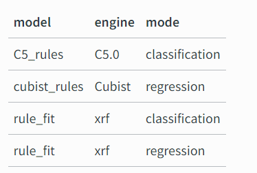
The rules package provides engines for the models in the following table.
# Model Specification
cubist_spec <-
  cubist_rules(
    committees = tune(),
    neighbors = tune(),
    max_rules = tune()
  )

# Workflow
library(rules)
cubist_wflow <-
  soc_wf %>%
  add_model(cubist_spec)

# Recipe
set.seed(1)
cubist_res <-
  tune_grid(
    object = cubist_wflow,
    resamples = cv_folds,
    grid = 20,
    control = ctrl_grid
)A Support Vector Machine (SVM) is a powerful supervised learning algorithm used for classification and regression tasks. SVMs are particularly effective when working with high-dimensional data and can handle both linear and non-linear relationships between variables.
The main idea behind SVM is to find an optimal hyperplane that separates data points of different classes with the largest possible margin. In other words, SVM tries to create a decision boundary that maximally separates the classes in the feature space. The data points that lie closest to the decision boundary are called support vectors.
install.packages(“kernlab”)
# # Model Specification
svm_spec <-
  svm_rbf(
    cost = tune(),
    rbf_sigma = tune()
  ) %>%
  set_engine("kernlab") %>%
  set_mode("regression")

# add it to a workflow
svm_wflow <-
  soc_wf %>%
  add_model(svm_spec)

# tune cost and rbf_sigma and fit to the 5-fold cv
set.seed(1)
svm_res <-
  tune_grid(
    svm_wflow,
    resamples = cv_folds,
    grid = 20,
    control = ctrl_grid
)A Neural Network (NN) is a type of artificial intelligence model inspired by the structure and functioning of the human brain. It is a powerful machine learning algorithm that can learn complex patterns and relationships in data to perform tasks such as classification, regression, pattern recognition, and more.
# Model Specification
nnet_spec <-
  mlp(
    hidden_units = tune(),
    penalty = tune(),
    epochs = tune()
  ) %>%
  set_mode("regression") %>%
  set_engine("nnet")

nnet_wflow <-
  soc_wf %>%
  add_model(nnet_spec)

nnet_res <-
  tune_grid(
    object = nnet_wflow,
    resamples = cv_folds,
    grid = 20,
    control = ctrl_grid
)We will use a simple function called finalizer() from here that selects the best model, updates the workflow, fits the final model with the best parameters and pulls out the metrics.
finalizer <- function(tuned, wkflow, split, model) {
  best_mod <- tuned %>%
    select_best("rmse")

  final_wf <- wkflow %>%
    finalize_workflow(best_mod)

  final_fit <-
    final_wf %>%
    last_fit(split)

  final_fit %>%
    collect_metrics() %>%
    mutate(model = model)
}
We have fitted 100 models, 20 models for each type (glm, random forest, lightgbm,cubist, and neural net). We can do a quick check of how well each of these models performed using finalize() function:
bind_rows(
  finalizer(glm_res, glm_wflow, split, "glm"),
  finalizer(rf_res, rf_wflow, split, "rf"),
  finalizer(lightgbm_res, lightgbm_wflow, split, "lightgbm"),
  finalizer(cubist_res, cubist_wflow, split, "cubist"),
  finalizer(svm_res, svm_wflow, split, "svm"),
  finalizer(nnet_res, nnet_wflow, split, "nnet"),
) %>%
  select(model, .metric, .estimate) %>%
  pivot_wider(names_from = .metric, values_from = .estimate) %>%
  arrange(rmse)
# A tibble: 6 × 3
model rmse rsq
<chr> <dbl> <dbl>
1 cubist 1.23 0.938
2 rf 1.40 0.923
3 lightgbm 2.82 0.681
4 svm 3.35 0.547
5 glm 3.82 0.406
6 nnet 10.3 0.182We can see that the cubist model has the best performance, followed by the rf.
First, we start by initialising the stack with stacks() then add each candidate model with add_candidates(). Next we evaluate the candidate models with blend_predictions(), before finally training the non-zero members on the training data with fit_members().
soc_stack <-
  # initialize the stack
  stacks() %>%
  # add each of the models
  add_candidates(glm_res) %>%
  add_candidates(rf_res) %>%
  add_candidates(lightgbm_res) %>%
  add_candidates(cubist_res) %>%
  add_candidates(svm_res) %>%
  add_candidates(nnet_res) %>%
  blend_predictions(penalty = range(c(0.5, 5),levels=50, mixture = 0), metric = metric_set(rmse)) %>% # evaluate candidate models
fit_members() # fit non zero stacking coefficientssoc_stack── A stacked ensemble model ─────────────────────────────────────
Out of 120 possible candidate members, the ensemble retained 8.
Penalty: 0.
Mixture: 1.
The 8 highest weighted members are:# A tibble: 8 × 3
member type weight
<chr> <chr> <dbl>
1 svm_res_1_09 svm_rbf 0.859
2 lightgbm_res_1_16 boost_tree 0.470
3 cubist_res_1_15 cubist_rules 0.440
4 rf_res_1_05 rand_forest 0.320
5 cubist_res_1_03 cubist_rules 0.276
6 lightgbm_res_1_07 boost_tree 0.116
7 lightgbm_res_1_14 boost_tree 0.00974
8 nnet_res_1_01 mlp 0.00497library(see) # for nice theme
autoplot(soc_stack, type = "weights") +
theme_lucid()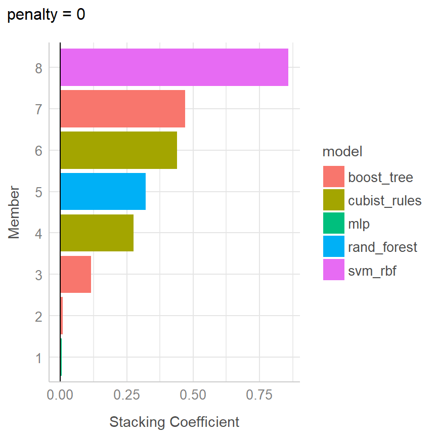
reg_metrics <- metric_set(rmse, rsq)
# get predictions with stack
soc_pred <- predict(soc_stack, test) %>%
bind_cols(test)ggplot(soc_pred, aes(x = SOC, y = .pred)) +
geom_point(alpha = 0.4) +
coord_obs_pred() +
labs(x = "Observed", y = "Predicted") +
geom_abline(linetype = "dashed") +
theme_lucid()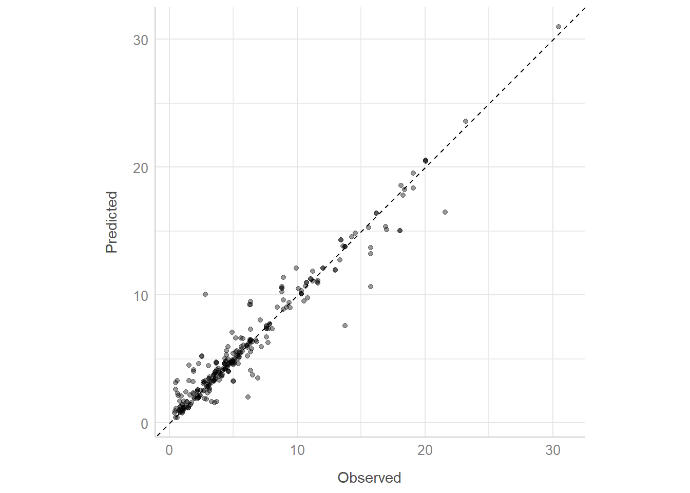
member_preds <-
  test %>%
  select(SOC) %>%
  bind_cols(
    predict(
      soc_stack,
      test,
      members = TRUE
    )
)colnames(member_preds) %>%
map_dfr(
.f = rmse,
truth = SOC,
data = member_preds
) %>%
mutate(member = colnames(member_preds))# A tibble: 10 × 4
.metric .estimator .estimate member
<chr> <chr> <dbl> <chr>
1 rmse standard 0 SOC
2 rmse standard 1.20 .pred
3 rmse standard 1.38 rf_res_1_05
4 rmse standard 4.93 lightgbm_res_1_16
5 rmse standard 4.93 lightgbm_res_1_07
6 rmse standard 4.93 lightgbm_res_1_14
7 rmse standard 1.45 cubist_res_1_03
8 rmse standard 1.26 cubist_res_1_15
9 rmse standard 5.15 svm_res_1_09
10 rmse standard 4.30 nnet_res_1_01 colnames(member_preds) %>%
map_dfr(
.f = rsq,
truth = SOC,
data = member_preds
) %>%
mutate(member = colnames(member_preds))# A tibble: 10 × 4
.metric .estimator .estimate member
<chr> <chr> <dbl> <chr>
1 rsq standard 1 SOC
2 rsq standard 0.941 .pred
3 rsq standard 0.927 rf_res_1_05
4 rsq standard 0.541 lightgbm_res_1_16
5 rsq standard 0.503 lightgbm_res_1_07
6 rsq standard 0.484 lightgbm_res_1_14
7 rsq standard 0.916 cubist_res_1_03
8 rsq standard 0.935 cubist_res_1_15
9 rsq standard 0.380 svm_res_1_09
10 rsq standard 0.377 nnet_res_1_01