Data Import-Export into/from R

Reading data for analysis and exporting the results to another system for report writing can be done efficiently with R. There are multiple ways to import and export data to/from R. In this tutorial, you will learn some most common ways to read and write data with R.

All data set use in this exercise can be downloaded from my dropbox folder.

Working directory

It would be best if you created a working directory in R to read and write files locally. The following example shows how to create the working directory in R.

Before creating a working directory, you may check the directory of your current R session; the function getwd() will print the current working directory path as a string.

Code

getwd()

[1] "F:/GitHub/R_QuartoWebsite/dsm"

If you want to change the working directory in R you just need to call the setwd() function, specifying as argument the path of the new working directory folder.

setwd(“F:\R-Project”)

setwd(“F:/R-Project”)

Remember that you must use the forward slash / or double backslash \ in R! The Windows format of single backslash will not work.

The files under in a directory can check using dir() function

dir()

Read/Import Data into R

Importing data using R-Studio IDE

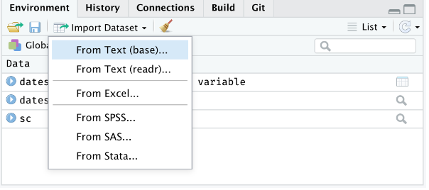
Importing data into R becomes time intensive. The easiest way to import data into R is by using RStudio IDE. This feature can be accessed from the Environment pane or from the **tools menu*. The importers are grouped into three categories: Text data, Excel data, and statistical data. The detail could be found here.

To access this feature, use the “Import Dataset” dropdown from the “Environment” pane:

Figure 1: Data Import RStudio Environment Pane

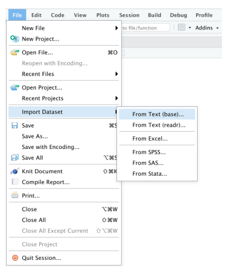
Or through the “File” menu, followed by the “Import Dataset” submenu:

Figure 2: Data Import RStudio File Menu

Text File (.txt)

The easiest form of data to import into R is a simple text file. The primary function to import from a text file is read.table().

read.table(file, header = FALSE, sep = ““, quote =”“’”,…..)

Code

# define data folder
dataFolder<-"E:/Dropbox/GitHub/Data/"
# read .txt file
df.txt<-read.table(paste0(dataFolder,"test_data.txt"), header= TRUE) 
#data.txt<-read.table("test_data.txt", header= TRUE) 
head(df.txt)

   ID treat  var rep    PH   TN   PN   GW ster   DTM   SW   GAs  STAs
1 Low    As BR01   1  84.0 28.3 27.7 35.7 20.5 126.0 28.4 0.762 14.60
2 Low    As BR01   2 111.7 34.0 30.0 58.1 14.8 119.0 36.7 0.722 10.77
3 Low    As BR01   3 102.3 27.7 24.0 44.6  5.8 119.7 32.9 0.858 12.69
4 Low    As BR06   1 118.0 23.3 19.7 46.4 20.3 119.0 40.0 1.053 18.23
5 Low    As BR06   2 115.3 16.7 12.3 19.9 32.3 120.0 28.2 1.130 13.72
6 Low    As BR06   3 111.0 19.0 15.3 35.9 14.9 116.3 42.3 1.011 15.97

Code

names(df.txt)

 [1] "ID"    "treat" "var"   "rep"   "PH"    "TN"    "PN"    "GW"    "ster" 
[10] "DTM"   "SW"    "GAs"   "STAs" 

However, scan() function could be used to scan and read data. It is usually used to read data into vector or list or from file in R Language.

sacn(scan(file = ““, what = double(), nmax = -1, n = -1, sep =”“,..)

Code

# define data folder
dataFolder<-"E:/Dropbox/GitHub/Data/"
# Scan data 
df.scan<-scan(paste0(dataFolder,"test_data.txt"),  what = list("", "", ""))   

Comma-Separated File (.csv)

A comma delimited or comma-separated file (CSV) is one where each value in the file is separated by a comma, although other characters can be used. Reading data from a CSV file is made easy by the read.csv(), an extension of read.table(). It facilitates the direct import of data from CSV files.

read.csv(file, header = TRUE, sep = “,”, quote = “““,…)

Code

# define data folder
dataFolder<-"E:/Dropbox/GitHub/Data/"
# read .csv file
df.csv<-read.csv(paste0(dataFolder,"test_data.csv"), header= TRUE) 
#head(data.csv)

Excel Files (.xlsx)

One of the best ways to read an Excel file is to export it to a comma-delimited file and import it using the method above. Alternatively, we can use the xlsx package to access Excel files. The first row should contain variable/column names.

install.packages(“xlsx”)

Code

# Load xlsx package
library(xlsx)
# define data folder
dataFolder<-"E:/Dropbox/GitHub/Data/"
# Import Sheet 1, from a excel file
data.xlsx <-xlsx::read.xlsx(paste0(dataFolder,"test_data.xlsx"), 1) 
#data.xlsx <-read.xlsx("test_data.xlsx", 1)  
names(data.xlsx)

 [1] "ID"    "treat" "var"   "rep"   "PH"    "TN"    "PN"    "GW"    "ster" 
[10] "DTM"   "SW"    "GAs"   "STAs" 

JSON Files (.json)

JSON is an open standard file and lightweight data-interchange format that stands for JavaScript Object Notation. The JSON file is a text file that is language independent, self-describing, and easy to understand.

The JSON file is read by R as a list using the function fromJSON() of rjson package.

install.packages(“rjson”)

fromJSON(json_str, file, method = “C”, unexpected.escape = “error”, sim..)

Code

# Load rjson package
library(rjson)
# define data folder
dataFolder<-"E:/Dropbox/GitHub/Data/"
# read .json file
df.json <- rjson::fromJSON(file= paste0(dataFolder, "test_data.json"),  simplify=TRUE)
#print(df.json)

We can convert to data frame

Code

df.json <- as.data.frame(df.json)
head(df.json)

  ID  treat  var rep    PH   TN   PN   GW ster   DTM   SW   GAs  STAs
1  1 Low As BR01   1  84.0 28.3 27.7 35.7 20.5 126.0 28.4 0.762 14.60
2  2 Low As BR01   2 111.7 34.0 30.0 58.1 14.8 119.0 36.7 0.722 10.77
3  3 Low As BR01   3 102.3 27.7 24.0 44.6  5.8 119.7 32.9 0.858 12.69
4  4 Low As BR06   1 118.0 23.3 19.7 46.4 20.3 119.0 40.0 1.053 18.23
5  5 Low As BR06   2 115.3 16.7 12.3 19.9 32.3 120.0 28.2 1.130 13.72
6  6 Low As BR06   3 111.0 19.0 15.3 35.9 14.9 116.3 42.3 1.011 15.97

Import Data from Other Stattistcal Software

foreign packages is mostly used to read data stored by Minitab, S, SAS, SPSS, Stata, Systat, dBase, and so forth.

install.packages(“foreign”)

Haven enables R to read and write various data formats used by other statistical packages by wrapping with ReadStat C library. written b Haven is part of the tidyverse. Current it support SAS, SPSS and Stata files

read.dta() function from foreign package can reads a file in Stata version 5-12 binary format (.dta) into a data frame.

STATA File (.dta)

Foreign - read.dta()

Code

# Load foreign package
library(foreign)
# define data folder
dataFolder<-"E:/Dropbox/GitHub/Data/"
# read .dta file
df.dta_01 <- foreign::read.dta(paste0(dataFolder,"test_data.dta")) 

Haven read_dta()

Code

# Load foreign package
library(haven)
# define data folder
dataFolder<-"E:/Dropbox/GitHub/Data/"
# read .dta file
df.dta_02 <- haven::read_dta(paste0(dataFolder,"test_data.dta")) 

SPSS File (.sav)

Foreign - read.spss()

Code

# Load foreign package
library(foreign)
# define data folder
dataFolder<-"E:/Dropbox/GitHub/Data/"
# read .sav file
df.sav_01 <- foreign::read.spss(paste0(dataFolder,"test_data.sav")) 

Haven read_sav()

Code

# Load haven package
library(haven)
# define data folder
dataFolder<-"E:/Dropbox/GitHub/Data/"
# read .sav file
df.sav_02 <- haven::read_sav(paste0(dataFolder,"test_data.sav")) 
#head(df.sav)

SAS File (.sas7bdat)

read_sas() function from haven package can read sas (.sas7bdat) file easily.

Code

# Load haven package
library(haven)
# define data folder
dataFolder<-"E:/Dropbox/GitHub/Data/"
# read .sas7bdat file
df.sas <- haven::read_sas(paste0(dataFolder,"test_data.sas7bdat")) 
#head(df.sas)

Export files from R

To export data and save to your local drive, you need the file path and an extension. First of all, the path is the location where the data will be stored.

Before we start, we need to specify the working directory in which we can export the data.

CSV File

First of all, let create a data frame that we will going to export as a text/CSV file.

Code

Variety =c("BR1","BR3", "BR16", "BR17", "BR18", "BR19","BR26",
          "BR27","BR28","BR29","BR35","BR36") # create a text vector
Yield = c(5.2,6.0,6.6,5.6,4.7,5.2,5.7,
                5.9,5.3,6.8,6.2,5.8) # create numerical vector
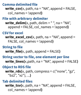
rice.data= data.frame(Variety, Yield)

The popular R base functions for writing data are write.table(), write.csv(), write.csv2() and write.delim() functions.

Before start, you need to specify the working or destination directory in where you will save the data.

Code

# Define destination folder
dataFolder<-"E:/Dropbox/GitHub/Data/"
write.csv(rice.data, paste0(dataFolder, "rice_data.csv"), row.names = F) # no row names
# write.csv(rice.data, "rice_data.csv", row.names = F) # no row names

Excel File

Exporting data from R to Excel can be achieved with several packages. The most known package to export data frames or tables as Excel is xlsx, that provides the write.xlsx and write.xlsx2 functions.

Code

# load xlsx
library(xlsx)
# Define destination folder
dataFolder<-"E:/Dropbox/GitHub/Data/"
# write as xlsx file
xlsx::write.xlsx(rice.data, paste0(dataFolder, "rice_data.xlsx"))

JSON Objects

To write JSON Object to file, the toJSON() function from the rjson library can be used to prepare a JSON object and then use the write() function for writing the JSON object to a local file.

Code

# Load rjson package
library(rjson)
# define data folder
dataFolder<-"E:/Dropbox/GitHub/Data/"
# create a JSON object
jsonData <-rjson::toJSON(rice.data)
# write JSON objects
write(jsonData, file= paste0(dataFolder,"rice_data.json"))

R Data File

If you want to share the data from R as Objects and share those with your colleagues through different systems so that they can use it right away into their R-workspace. These objects are of two types .rda/.RData which can be used to store some or all objects, functions from R global environment.

The save() function allows us to save multiple objects into our global environment:

Note

If you specify save.image(file = “R_objects.RData”) Export all objects (the workspace image).

To save only one object it is more recommended saving it as RDS with the saveRDS() function:

Code

# write .RDS file
saveRDS(rice.data, "E:/Dropbox/GitHub/Data/rice_data.rds")

Note

If you specify compress = TRUE as argument of the above functions the file will be compressed by default as gzip.

Export to Other Statistcal Software

STATA File

If you want export data from R to STATA, you will need to use the write.dta() function of the foreign package. This package provides functions for r

Code

# Load foreign package
library(foreign)
# define data folder
dataFolder<-"E:/Dropbox/GitHub/Data/"
# write dta file
foreign::write.dta(rice.data, file= paste0(dataFolder,"rice_data.dta"))

SPSS File

Haven enables R to read and write various data formats used by other statistical packages by wrapping with ReadStat C library. written b Haven is part of the tidyverse. Current it support SAS, SPSS and Stata files

The write_sav() function of haven package can be used to export R-object to SPSS

Code

# Load haven package
library(haven)
# write .sav file
haven::write_sav(rice.data, "E:/Dropbox/GitHub/Data/rice_data.sav")

SAS File

The write_sas() function of haven package can be used to export R-object to SAS (.sas7bdat)

Code

# Load haven package
library(haven)
# write .sav file
haven::write_sas(rice.data, "E:/Dropbox/GitHub/Data/rice_data.sas7bdat")

data.table: Extension of ‘data.frame’

The R-package data.tabel a improved version of data.frame, the a R-base function. It has following advantages:

• concise syntax: fast to type, fast to read • fast speed • memory efficient

install.packages(“data.table”)

We will use two important functions of data.table to read and write CSV files in R.

Reaing CSV file with fread

fread: This function is capable of reading CSV files quickly and conveniently.

fread(input, file,….)

Code

# Load library
library(data.table)
# define data location
dataFolder<-"E:/Dropbox/GitHub/Data/"
# read with fread()
DT<-data.table::fread(paste0(dataFolder,"LBC_data.csv"), header= TRUE) 
str(DT)

Classes 'data.table' and 'data.frame':  3110 obs. of  25 variables:
 $ REGION_ID         : int  3 3 3 3 3 3 3 3 3 3 ...
 $ STATE             : chr  "Alabama" "Alabama" "Alabama" "Alabama" ...
 $ County            : chr  "Baldwin County" "Butler County" "Butler County" "Chambers County" ...
 $ Empty Column 1    : logi  NA NA NA NA NA NA ...
 $ X                 : num  789778 877732 877732 984215 726606 ...
 $ Y                 : num  884557 1007286 1007286 1148649 1023616 ...
 $ Fips              : int  1003 1013 1013 1017 1023 1025 1031 1035 1039 1041 ...
 $ LCB Mortality Rate: num  48.1 38.3 38.3 49.6 31.8 42 53.7 46.9 65.5 57.1 ...
 $ Smoking           : num  20.8 26 26 25.1 21.8 22.6 21.2 24.9 25.9 22.9 ...
 $ PM  25            : num  7.89 8.46 8.46 8.87 8.58 8.42 8.42 8.23 8.24 8.45 ...
 $ NO2               : num  0.794 0.634 0.634 0.844 0.593 ...
 $ SO2               : num  0.0353 0.0135 0.0135 0.0482 0.024 ...
 $ Ozone             : num  39.8 38.3 38.3 40.1 37.1 ...
 $ Pop 65            : num  19.5 19 19 18.9 22.1 19 16.3 21.6 20.5 18.3 ...
 $ Pop Black         : num  9.24 43.94 43.94 39.24 41.94 ...
 $ Pop Hipanic       : num  4.54 1.26 1.26 2.14 0.86 1.34 6.76 1.84 1.62 1.86 ...
 $ Pop White         : num  83.1 52.6 52.6 56.4 56.3 ...
 $ Education         : int  66 38 38 47 55 39 60 35 53 44 ...
 $ Poverty %         : num  13.1 26.1 26.1 21.5 23.1 ...
 $ Income Equality   : num  4.5 5.1 5.1 4.7 5.8 8.2 4.8 4.9 4.6 5.8 ...
 $ Uninsured         : num  13.3 12.7 12.7 13.3 12.9 ...
 $ DEM               : num  36.8 111.7 111.7 227 68.2 ...
 $ Radon Zone Class  : chr  "Zone-3" "Zone-3" "Zone-3" "Zone-3" ...
 $ Urban Rural       : chr  "Medium/small metro" "Nonmetro" "Nonmetro" "Nonmetro" ...
 $ Coal Production   : chr  "No" "No" "No" "No" ...
 - attr(*, ".internal.selfref")=<externalptr> 

Code

#DT<-fread("usa_geochemical.csv", header= TRUE) 

You cam compare data reading time of fread() and read.csv() functions:

R-base function read.csv

Code

system.time(read.csv(paste0(dataFolder,"LBC_data.csv"), header= TRUE)) 

   user  system elapsed 
   0.05    0.00    0.05 

data.table fread

Code

system.time(data.table::fread(paste0(dataFolder,"LBC_data.csv"), header= TRUE))

   user  system elapsed 
      0       0       0 

Writing CSV file with fwrite

fwrite(): This capable to write CSV field very fast!

fwrite(x, file = ““, append = FALSE, quote =”auto”, …..)

Code

# define data location
dataFolder<-"E:/Dropbox/GitHub/Data/"
# read with fread()
data.table::fwrite(DT,  paste0(dataFolder, "DT.csv"), row.names=F, quote=TRUE)

Now we compare writing time of frwite functions with write.csv functions.

R-base function write.csv

Code

system.time(write.csv(DT,  paste0(dataFolder, "DT.csv"), row.names=F))

user system elapsed 0.2 0.0 0.2

data.table fwrite

Code

system.time(data.table::fwrite(DT,  paste0(dataFolder, "DT.csv"), row.names=F, quote=TRUE))

   user  system elapsed 
   0.01    0.00    0.02 

Feather: A Fast On-Disk Format for Data Frames

Feather is a fast, lightweight, and easy-to-use binary file format for storing data frames. It has a few specific design goals:

• Lightweight, minimal API: make pushing data frames in and out of memory as simple as possible

• Language agnostic: Feather files are the same whether written by Python or R code. Other languages can read and write Feather files, too.

Feather is extremely fast. Since Feather does not currently use any compression internally, it works best when used with solid-state drives as come with most of today’s laptop computers. For this first release, we prioritized a simple implementation and are thus writing unmodified Arrow memory to disk source.

install.packages(“feather”)

Code

#install.packages("feather")
library(feather)

First we have to create feather data using write_feather() function

write_feather(x, path)

Code

# define data location
dataFolder<-"E:/Dropbox/GitHub/Data/"
# Load feather
library(feather)
# write_feather()
feather::write_feather(DT, paste0(dataFolder, "LBC_data.feather"))

We can read this feather data with lighting speed using read_feather function()

Code

DT_feather <- feather::read_feather(paste0(dataFolder, "LBC_data.feather"))
str(DT_feather)

tibble [3,110 × 25] (S3: tbl_df/tbl/data.frame)
 $ REGION_ID         : int [1:3110] 3 3 3 3 3 3 3 3 3 3 ...
 $ STATE             : chr [1:3110] "Alabama" "Alabama" "Alabama" "Alabama" ...
 $ County            : chr [1:3110] "Baldwin County" "Butler County" "Butler County" "Chambers County" ...
 $ Empty Column 1    : logi [1:3110] NA NA NA NA NA NA ...
 $ X                 : num [1:3110] 789778 877732 877732 984215 726606 ...
 $ Y                 : num [1:3110] 884557 1007286 1007286 1148649 1023616 ...
 $ Fips              : int [1:3110] 1003 1013 1013 1017 1023 1025 1031 1035 1039 1041 ...
 $ LCB Mortality Rate: num [1:3110] 48.1 38.3 38.3 49.6 31.8 42 53.7 46.9 65.5 57.1 ...
 $ Smoking           : num [1:3110] 20.8 26 26 25.1 21.8 22.6 21.2 24.9 25.9 22.9 ...
 $ PM  25            : num [1:3110] 7.89 8.46 8.46 8.87 8.58 8.42 8.42 8.23 8.24 8.45 ...
 $ NO2               : num [1:3110] 0.794 0.634 0.634 0.844 0.593 ...
 $ SO2               : num [1:3110] 0.0353 0.0135 0.0135 0.0482 0.024 ...
 $ Ozone             : num [1:3110] 39.8 38.3 38.3 40.1 37.1 ...
 $ Pop 65            : num [1:3110] 19.5 19 19 18.9 22.1 19 16.3 21.6 20.5 18.3 ...
 $ Pop Black         : num [1:3110] 9.24 43.94 43.94 39.24 41.94 ...
 $ Pop Hipanic       : num [1:3110] 4.54 1.26 1.26 2.14 0.86 1.34 6.76 1.84 1.62 1.86 ...
 $ Pop White         : num [1:3110] 83.1 52.6 52.6 56.4 56.3 ...
 $ Education         : int [1:3110] 66 38 38 47 55 39 60 35 53 44 ...
 $ Poverty %         : num [1:3110] 13.1 26.1 26.1 21.5 23.1 ...
 $ Income Equality   : num [1:3110] 4.5 5.1 5.1 4.7 5.8 8.2 4.8 4.9 4.6 5.8 ...
 $ Uninsured         : num [1:3110] 13.3 12.7 12.7 13.3 12.9 ...
 $ DEM               : num [1:3110] 36.8 111.7 111.7 227 68.2 ...
 $ Radon Zone Class  : chr [1:3110] "Zone-3" "Zone-3" "Zone-3" "Zone-3" ...
 $ Urban Rural       : chr [1:3110] "Medium/small metro" "Nonmetro" "Nonmetro" "Nonmetro" ...
 $ Coal Production   : chr [1:3110] "No" "No" "No" "No" ...

Compare to and write.csv() as well as frwite(), write_feather() is very fast:

R-base write.csv

Code

system.time(write.csv(DT, paste0(dataFolder, "LBC_data.csv")))

   user  system elapsed 
   0.23    0.00    0.24 

data.table fwrite

Code

# CSV file with fwrite
system.time(data.table::fwrite(DT, paste0(dataFolder, "LBC_data.csv")))

   user  system elapsed 
   0.02    0.00    0.02 

Feather write_feather

Code

# feather file with 
system.time(feather::write_feather(DT, paste0(dataFolder, "LBC_data.feather")))

   user  system elapsed 
      0       0       0 

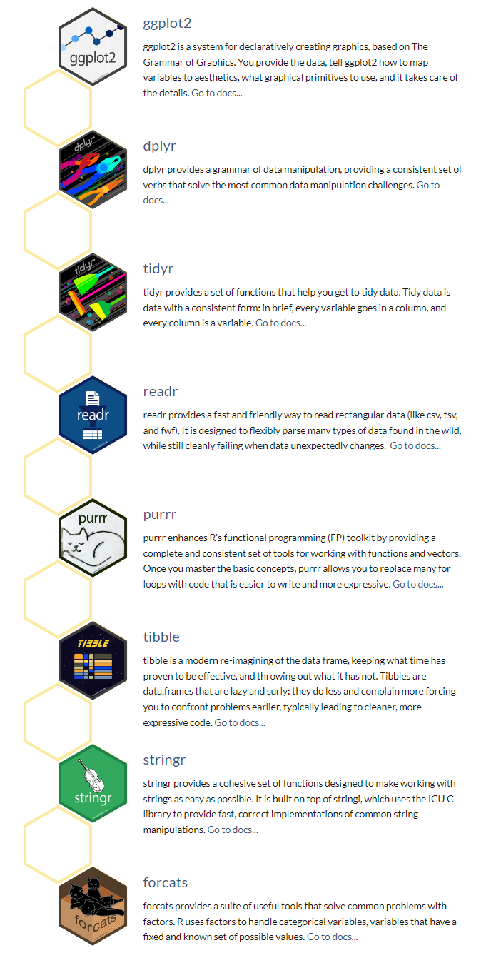
Tidyverse Package: Data Import and Export

The tidyverse is an collection of several R packages designed for data science. All packages share an underlying design philosophy, grammar, and data structures (Source).

The core tidyverse includes the packages that you’re likely to use in everyday data analyses. As of tidyverse 1.3.0, the following packages are included in the core tidyverse:

Figure 3: Core R-Packages

Installation and use

• Install all the packages in the tidyverse by running install.packages(“tidyverse”).

• Run library(tidyverse) to load the core tidyverse with and make it available in your current R session.

install.packages(“tidyverse”)

Code

library(tidyverse)

As well as readr, for reading flat files, the tidyverse package installs a number of other packages for reading data:

• DBI for relational databases. You’ll need to pair DBI with a database specific backends like RSQLite, RMariaDB, RPostgres, or odbc. Learn more at https://db.rstudio.com.

• haven for SPSS, Stata, and SAS data.

• httr for web APIs.

• readxl for .xls and .xlsx sheets.

• googlesheets4 for Google Sheets via the Sheets API v4.

• googledrive for Google Drive files.

• rvest for web scraping.

• jsonlite for JSON. (Maintained by Jeroen Ooms.)

• xml2 for XML

Read CSV files with readr

A tibble, or tbl_df, is the latest method for reimagining of modern data-frame and It keeps all the crucial features regarding the data frame. Since R is an old language, and some things that were useful 10 or 20 years ago now get in your way. It’s difficult to change base R without breaking existing code, so most innovation occurs in tibble() data-frame with tibble package.

Key features of Tibble

• A Tibble never alters the input type.

• With Tibble, there is no need for us to be bothered about the automatic changing of characters to strings.

• Tibbles can also contain columns that are the lists.

• We can also use non-standard variable names in Tibble.

• We can start the name of a Tibble with a number, or we can also contain space.

• To utilize these names, we must mention them in backticks.

• Tibble only recycles the vectors with a length of 1.

• Tibble can never generate the names of rows.

source: https://www.educative.io/answers/what-is-tibble-versus-data-frame-in-r

We can use following functions readr package to import tabular data into R as tibble:

Figure 4: read() Functions

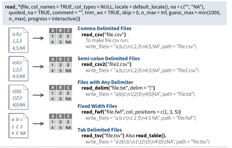
read_csv() and read_tsv() are special cases of the more general read_delim(). They’re useful for reading the most common types of flat file data, comma separated values and tab separated values, respectively. read_csv2() uses ⁠;⁠ for the field separator and ⁠,⁠ for the decimal point. This format is common in some European countries.

For example, we will use read_csv() to import CSV file and see use glimpse() functions of dplyr package to explore the file structure.

read_csv()

Code

# define data location
dataFolder<-"E:/Dropbox/GitHub/Data/"
df.chem_01<-readr::read_csv(paste0(dataFolder,"PAHdata.csv"))

Rows: 20 Columns: 23
── Column specification ────────────────────────────────────────────────────────
Delimiter: ","
chr  (1): Subject
dbl (22): Napthalene, 1-Methyl Napthalene, 2-Methyl Napthalene, Acenapthylen...

ℹ Use `spec()` to retrieve the full column specification for this data.
ℹ Specify the column types or set `show_col_types = FALSE` to quiet this message.

Code

dplyr::glimpse(df.chem_01)

Rows: 20 Columns: 23 $ Subject “P1”, “P3”, “P4”, “P5”, “P6”, “P7”, “P8”, … $ Napthalene 0.8993, 3.6257, 3.3921, 3.5772, 4.4907, NA… $ 1-Methyl Napthalene 4.9681, 4.6941, 3.5386, 4.7475, 5.1147, NA… $ 2-Methyl Napthalene 2.1508, 3.9316, 1.6955, 2.9361, 3.9976, NA… $ Acenapthylene 0.0131, 3.0151, 1.3859, 3.3943, 6.6593, NA… $ 1,2 Dimethyl napthalene NA, NA, 1.2389, 2.6427, 2.1442, NA, 0.3623… $ 1,6 Dimethyl Napthalene 0.7003, 2.6382, 1.3807, 1.1006, 2.2575, NA… $ Fluorene 2.2481, 7.3490, 7.1567, 8.4422, 9.2363, NA… $ 1,6,7 Trimethylnapthalene 5.1024, 6.7913, 6.5171, 4.6803, 6.4649, NA… $ Anthracene 10.1656, 9.6419, 22.3997, 26.3787, 20.9594… $ Dibenzothiopene 1.1633, 4.1160, 4.2256, 3.9885, 3.2560, NA… $ 2-Methyl Anthracene 0.5409, 4.5190, 8.4014, 13.0101, 4.4900, N… $ 1-Methylphenanthrene 14.9581, 12.0937, 19.4927, 11.2138, 2.0336… $ 2-Methylphenanthrene 5.4785, 18.2456, 36.4282, 16.4553, 10.8040… $ Pyrene 4.8498, 14.9369, 10.1099, 26.0579, 20.8687… $ Fluoranthene 4.4798, 9.7189, 9.8037, 19.0489, 20.0866, … $ 1-Phenyl napthalene 2.8778, 6.2493, 5.2998, 7.9514, 10.1570, N… $ 2-Phenyl napthalene 3.4092, 8.7412, 3.6956, 12.8510, 15.1037, … $ 1 Methylpyrene 4.5763, 7.5114, 13.6010, 8.1125, 19.2354, … $ Benzo(c)phenanthrene 3.6456, 7.0372, 5.0960, 3.3828, 8.1571, NA… $ Triphenylene/Chrysene 1.7422, 5.1389, 3.1635, 5.7081, 6.7483, NA… $ Benz(a)pyrene NA, 2.8455, NA, 5.0701, 0.5873, NA, 9.0914… $ Benz(e)pyrene NA, 1.8163, 0.2980, 0.6617, 2.3666, NA, 2.…

read.csv()

Code

# define data location
dataFolder<-"E:/Dropbox/GitHub/Data/"
df.chem_02<-read.csv(paste0(dataFolder,"PAHdata.csv"))
dplyr::glimpse(df.chem_02)

Rows: 20
Columns: 23
$ Subject                    <chr> "P1", "P3", "P4", "P5", "P6", "P7", "P8", "…
$ Napthalene                 <dbl> 0.8993, 3.6257, 3.3921, 3.5772, 4.4907, NA,…
$ X1.Methyl.Napthalene       <dbl> 4.9681, 4.6941, 3.5386, 4.7475, 5.1147, NA,…
$ X2.Methyl.Napthalene       <dbl> 2.1508, 3.9316, 1.6955, 2.9361, 3.9976, NA,…
$ Acenapthylene              <dbl> 0.0131, 3.0151, 1.3859, 3.3943, 6.6593, NA,…
$ X1.2.Dimethyl.napthalene   <dbl> NA, NA, 1.2389, 2.6427, 2.1442, NA, 0.3623,…
$ X1.6.Dimethyl.Napthalene   <dbl> 0.7003, 2.6382, 1.3807, 1.1006, 2.2575, NA,…
$ Fluorene                   <dbl> 2.2481, 7.3490, 7.1567, 8.4422, 9.2363, NA,…
$ X1.6.7.Trimethylnapthalene <dbl> 5.1024, 6.7913, 6.5171, 4.6803, 6.4649, NA,…
$ Anthracene                 <dbl> 10.1656, 9.6419, 22.3997, 26.3787, 20.9594,…
$ Dibenzothiopene            <dbl> 1.1633, 4.1160, 4.2256, 3.9885, 3.2560, NA,…
$ X2.Methyl.Anthracene       <dbl> 0.5409, 4.5190, 8.4014, 13.0101, 4.4900, NA…
$ X1.Methylphenanthrene      <dbl> 14.9581, 12.0937, 19.4927, 11.2138, 2.0336,…
$ X2.Methylphenanthrene      <dbl> 5.4785, 18.2456, 36.4282, 16.4553, 10.8040,…
$ Pyrene                     <dbl> 4.8498, 14.9369, 10.1099, 26.0579, 20.8687,…
$ Fluoranthene               <dbl> 4.4798, 9.7189, 9.8037, 19.0489, 20.0866, N…
$ X1.Phenyl.napthalene       <dbl> 2.8778, 6.2493, 5.2998, 7.9514, 10.1570, NA…
$ X2.Phenyl.napthalene       <dbl> 3.4092, 8.7412, 3.6956, 12.8510, 15.1037, N…
$ X1.Methylpyrene            <dbl> 4.5763, 7.5114, 13.6010, 8.1125, 19.2354, N…
$ Benzo.c.phenanthrene       <dbl> 3.6456, 7.0372, 5.0960, 3.3828, 8.1571, NA,…
$ Triphenylene.Chrysene      <dbl> 1.7422, 5.1389, 3.1635, 5.7081, 6.7483, NA,…
$ Benz.a.pyrene              <dbl> NA, 2.8455, NA, 5.0701, 0.5873, NA, 9.0914,…
$ Benz.e.pyrene              <dbl> NA, 1.8163, 0.2980, 0.6617, 2.3666, NA, 2.6…

Note

glimps() of dplyr is a improved function of r-base str() function.

Write CSV files with readr

The write()⁠ family functions of are an improvement to analogous function such as write.csv() because they are approximately twice as fast. Unlike write.csv(), these functions do not include row names as a column in the written file. A generic function, output_column(), is applied to each variable to coerce columns to suitable output.

We can use following functions readr package to extort tabular data from R:

Figure 5: write() Functions

Code

readr::write_csv(df.chem_02, "df.chem_02")

We can also use as_tibble() function of tibble package

Code

df.chem_03<-tibble::as_tibble(read.csv(paste0(dataFolder,"PAHdata.csv"), check.names = FALSE))
str(df.chem_03)

tibble [20 × 23] (S3: tbl_df/tbl/data.frame)
 $ Subject                  : chr [1:20] "P1" "P3" "P4" "P5" ...
 $ Napthalene               : num [1:20] 0.899 3.626 3.392 3.577 4.491 ...
 $ 1-Methyl Napthalene      : num [1:20] 4.97 4.69 3.54 4.75 5.11 ...
 $ 2-Methyl Napthalene      : num [1:20] 2.15 3.93 1.7 2.94 4 ...
 $ Acenapthylene            : num [1:20] 0.0131 3.0151 1.3859 3.3943 6.6593 ...
 $ 1,2 Dimethyl napthalene  : num [1:20] NA NA 1.24 2.64 2.14 ...
 $ 1,6 Dimethyl Napthalene  : num [1:20] 0.7 2.64 1.38 1.1 2.26 ...
 $ Fluorene                 : num [1:20] 2.25 7.35 7.16 8.44 9.24 ...
 $ 1,6,7 Trimethylnapthalene: num [1:20] 5.1 6.79 6.52 4.68 6.46 ...
 $ Anthracene               : num [1:20] 10.17 9.64 22.4 26.38 20.96 ...
 $ Dibenzothiopene          : num [1:20] 1.16 4.12 4.23 3.99 3.26 ...
 $ 2-Methyl Anthracene      : num [1:20] 0.541 4.519 8.401 13.01 4.49 ...
 $ 1-Methylphenanthrene     : num [1:20] 14.96 12.09 19.49 11.21 2.03 ...
 $ 2-Methylphenanthrene     : num [1:20] 5.48 18.25 36.43 16.46 10.8 ...
 $ Pyrene                   : num [1:20] 4.85 14.94 10.11 26.06 20.87 ...
 $ Fluoranthene             : num [1:20] 4.48 9.72 9.8 19.05 20.09 ...
 $ 1-Phenyl napthalene      : num [1:20] 2.88 6.25 5.3 7.95 10.16 ...
 $ 2-Phenyl napthalene      : num [1:20] 3.41 8.74 3.7 12.85 15.1 ...
 $ 1 Methylpyrene           : num [1:20] 4.58 7.51 13.6 8.11 19.24 ...
 $ Benzo(c)phenanthrene     : num [1:20] 3.65 7.04 5.1 3.38 8.16 ...
 $ Triphenylene/Chrysene    : num [1:20] 1.74 5.14 3.16 5.71 6.75 ...
 $ Benz(a)pyrene            : num [1:20] NA 2.845 NA 5.07 0.587 ...
 $ Benz(e)pyrene            : num [1:20] NA 1.816 0.298 0.662 2.367 ...

Further Reading

1. How do I read data into R?

2. R Coder

3. Introduction to bioinformatics

4. Many Ways of Reading Data Into R — 1

5. readr

6. feather

7. data.tabler

8. foreign

9. haven