Extreme Gradient Boosting (XGBoost)

XGBoost (Extreme Gradient Boosting) is a popular open-source machine learning library that is used to build gradient boosting models. It was first introduced in 2016 and has since become one of the most widely used and highly regarded machine learning algorithms for structured data.

The XGBoost algorithm works by building a series of decision trees, where each subsequent tree tries to correct the errors of the previous tree. The algorithm also employs a gradient-based optimization approach to find the optimal set of parameters for each decision tree.

XGBoost has several key features that make it popular among data scientists and machine learning practitioners. Firstly, it can handle missing values in the data, which is a common problem in real-world datasets. Secondly, it supports parallel processing, which makes it scalable and efficient for large datasets. Thirdly, it has built-in support for regularization, which helps to prevent overfitting and improve the generalization performance of the model. Finally, it provides a variety of evaluation metrics to measure the performance of the model, including accuracy, precision, recall, and F1 score.

Overall, XGBoost is a powerful and versatile machine learning algorithm that can be used for a wide range of structured data problems, including classification, regression, and ranking. Its ability to handle missing values, support parallel processing, and provide regularization makes it an excellent choice for building accurate and scalable machine learning models.

The XGBoost algorithm works as follows:

Initialize the model with a single decision tree.
Calculate the error between the predicted values and the actual values for each sample in the training dataset.
Train a new decision tree to predict the errors of the previous tree.
Add the new tree to the model and update the predicted values by summing the predictions of all the trees in the model.
Repeat steps 2 to 4 until the model reaches a certain level of accuracy, or until a maximum number of trees is reached.

Differences between LightGBM vs XGBoost

LightGBM (Light Gradient Boosting Machine) and XGBoost (Extreme Gradient Boosting) are both gradient boosting algorithms that are widely used in machine learning. While they share many similarities, there are some key differences between the two algorithms:

Speed: LightGBM is generally faster than XGBoost. This is because it uses a more efficient algorithm for finding the best split points, and it employs parallel processing to speed up the training process.
Scalability: LightGBM is more scalable than XGBoost. It can handle larger datasets with higher dimensional features, and it has a smaller memory footprint than XGBoost.
Handling missing values: LightGBM has built-in support for handling missing values in the data, which can be a common problem in real-world datasets. XGBoost also supports handling missing values, but it requires the user to manually specify the missing value handling strategy.
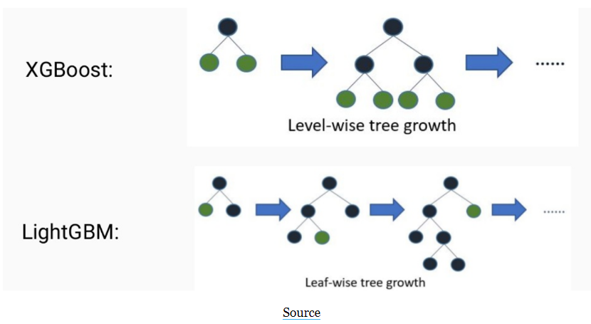
Leaf-wise growth: LightGBM uses a “Leaf-wise” growth strategy, which grows the tree by splitting the leaf that yields the maximum reduction in the loss function, resulting in a more balanced and less deep tree. XGBoost uses a “Level-wise” growth strategy, which grows the tree level-by-level, resulting in a deeper and more unbalanced tree.

Regularization: XGBoost provides more regularization options than LightGBM, which can help prevent overfitting and improve the generalization performance of the model.
Categorical features: LightGBM has built-in support for handling categorical features, which can be a common feature type in real-world datasets. XGBoost also supports categorical features, but it requires the user to manually encode the categorical variables.

Extreme Gradient Boosting with “XGBoost” package

The XGBoost package in R provides an implementation of the XGBoost algorithm, a powerful and flexible gradient boosting framework. Here are some key features of the XGBoost R package:

High performance: XGBoost is designed to be highly efficient and scalable, making it well-suited for large datasets and high-dimensional feature spaces. The R package provides an interface to the underlying C++ library, which allows it to take advantage of multi-threading and other optimization techniques.
Cross-validation: The XGBoost R package provides tools for cross-validation, which can be used to tune hyperparameters and assess model performance.
Feature importance: XGBoost computes the feature importance by measuring the number of times each feature is split on in the tree building process. The more a feature is used for splitting, the more important it is considered to be. The R package provides functions for visualizing the feature importance and selecting the most important features.
Regularization: XGBoost provides several regularization techniques, such as L1 and L2 regularization, to prevent overfitting. The R package provides options for controlling the amount of regularization.
Missing value handling: XGBoost can handle missing values in the data, using a default direction at each node to handle missing values.
Flexibility: XGBoost can be used for a wide range of machine learning tasks, including regression, classification, and ranking. It can also handle both numerical and categorical features, and supports custom objective functions.

Install the XGBoost R package from CRAN using the following command:

install.packages(“xgboost”)

Code

library(xgboost)

Data

In this exercise we will use following data set and use DEM, MAP, MAT, NAVI, NLCD, and FRG to fit XGBoost regression model.

gp_soil_data.csv

Code

library(tidyverse)
# define data folder
urlfile = "https://github.com//zia207/r-colab/raw/main/Data/USA/gp_soil_data.csv"
mf<-read_csv(url(urlfile))
# Create a data-frame
df<-mf %>% dplyr::select(SOC, DEM, Slope, Aspect, TPI, KFactor, SiltClay, MAT, MAP,NDVI, NLCD, FRG)%>%
    glimpse()

Rows: 467
Columns: 12
$ SOC      <dbl> 15.763, 15.883, 18.142, 10.745, 10.479, 16.987, 24.954, 6.288…
$ DEM      <dbl> 2229.079, 1889.400, 2423.048, 2484.283, 2396.195, 2360.573, 2…
$ Slope    <dbl> 5.6716146, 8.9138117, 4.7748051, 7.1218114, 7.9498644, 9.6632…
$ Aspect   <dbl> 159.1877, 156.8786, 168.6124, 198.3536, 201.3215, 208.9732, 2…
$ TPI      <dbl> -0.08572358, 4.55913162, 2.60588670, 5.14693117, 3.75570583, …
$ KFactor  <dbl> 0.31999999, 0.26121211, 0.21619999, 0.18166667, 0.12551020, 0…
$ SiltClay <dbl> 64.84270, 72.00455, 57.18700, 54.99166, 51.22857, 45.02000, 5…
$ MAT      <dbl> 4.5951686, 3.8599243, 0.8855000, 0.4707811, 0.7588266, 1.3586…
$ MAP      <dbl> 468.3245, 536.3522, 859.5509, 869.4724, 802.9743, 1121.2744, …
$ NDVI     <dbl> 0.4139390, 0.6939532, 0.5466033, 0.6191013, 0.5844722, 0.6028…
$ NLCD     <chr> "Shrubland", "Shrubland", "Forest", "Forest", "Forest", "Fore…
$ FRG      <chr> "Fire Regime Group IV", "Fire Regime Group IV", "Fire Regime …

Data Preparation

Code

library(fastDummies)
tmp <- df[, c(11:12)]
# create dummy variables
tmp1 <- dummy_cols(tmp)
tmp1 <- tmp1[,3:12]

# create a dataframe
d <- data.frame(df[, c(1:10)], tmp1)
m <- as.matrix(d)

Create training and test dataset

Code

library(caret)
set.seed(123)
indices <- sample(1:nrow(df), size = 0.75 * nrow(df))
train <- m[indices,]
test <- m[-indices,]

Load the train and test data into the xgboost dataset object

Code

#define predictor and response variables in training set
train_x = data.matrix(train[, -1])
train_y = train[,1]

#define predictor and response variables in testing set
test_x = data.matrix(test[, -1])
test_y = test[, 1]

#define final training and testing sets
xgb_train = xgb.DMatrix(data = train_x, label = train_y)
xgb_test = xgb.DMatrix(data = test_x, label = test_y)

Fit XGBoost model

Next, we’ll fit the XGBoost model by using the xgb.train() function, which displays the training and testing RMSE (root mean squared error) for each round of boosting. We use a few tunning prameters with default values.

Code

#define watchlist
watchlist = list(train=xgb_train, 
                 test=xgb_test)

#fit XGBoost model and display training and testing data at each round
xgboost_model = xgb.train(
                data = xgb_train, 
                max.depth = 6,          # max_depth maximum depth of a tree
                eta = 0.3,                  # eta control learning rate              
                nround = 1000,          # max number of boosting iterations.
                watchlist = watchlist, 
                objective = "reg:linear",     # objective specify the learning task 
                early_stopping_rounds = 100, # round for early stopping 
                print_every_n = 500)

[22:49:25] WARNING: src/objective/regression_obj.cu:213: reg:linear is now deprecated in favor of reg:squarederror.
[1] train-rmse:5.845926 test-rmse:6.275015 
Multiple eval metrics are present. Will use test_rmse for early stopping.
Will train until test_rmse hasn't improved in 100 rounds.

Stopping. Best iteration:
[7] train-rmse:2.065355 test-rmse:4.134119

Code

xgboost_model

##### xgb.Booster
raw: 269.8 Kb 
call:
  xgb.train(data = xgb_train, nrounds = 1000, watchlist = watchlist, 
    print_every_n = 500, early_stopping_rounds = 100, max.depth = 6, 
    eta = 0.3, objective = "reg:linear")
params (as set within xgb.train):
  max_depth = "6", eta = "0.3", objective = "reg:linear", validate_parameters = "TRUE"
xgb.attributes:
  best_iteration, best_msg, best_ntreelimit, best_score, niter
callbacks:
  cb.print.evaluation(period = print_every_n)
  cb.evaluation.log()
  cb.early.stop(stopping_rounds = early_stopping_rounds, maximize = maximize, 
    verbose = verbose)
# of features: 19 
niter: 107
best_iteration : 7 
best_ntreelimit : 7 
best_score : 4.134119 
best_msg : [7]  train-rmse:2.065355 test-rmse:4.134119 
nfeatures : 19 
evaluation_log:
    iter train_rmse test_rmse
       1  5.8459262  6.275015
       2  4.5774327  5.383818
---                          
     106  0.1186750  4.543295
     107  0.1185662  4.543125

Prediction

Code

yhat_fit_base <- predict(xgboost_model,train[,2:20])
yhat_predict_base <- predict(xgboost_model,test[,2:20])

Code

rmse_fit_base <- RMSE(train_y,yhat_fit_base)
rmse_predict_base <- RMSE(test_y,yhat_predict_base)
rmse_fit_base

[1] 2.065355

Code

rmse_predict_base

[1] 4.134118

Code

rm(list = ls())

Tunning XGBoost with tidymodel

The tidymodels provides a comprehensive framework for building, tuning, and evaluating XGBoost model while following the principles of the tidyverse.

Data

Code

library(tidyverse)
# define data folder
dataFolder<-"E:/Dropbox/GitHub/Data/USA/"
# Load data
mf<-read_csv(paste0(dataFolder, "gp_soil_data.csv"))
# Create a data-frame
df<-mf %>% dplyr::select(SOC, DEM, Slope, Aspect, TPI, KFactor, SiltClay, MAT, MAP,NDVI, NLCD, FRG)%>%
    glimpse()

Rows: 467
Columns: 12
$ SOC      <dbl> 15.763, 15.883, 18.142, 10.745, 10.479, 16.987, 24.954, 6.288…
$ DEM      <dbl> 2229.079, 1889.400, 2423.048, 2484.283, 2396.195, 2360.573, 2…
$ Slope    <dbl> 5.6716146, 8.9138117, 4.7748051, 7.1218114, 7.9498644, 9.6632…
$ Aspect   <dbl> 159.1877, 156.8786, 168.6124, 198.3536, 201.3215, 208.9732, 2…
$ TPI      <dbl> -0.08572358, 4.55913162, 2.60588670, 5.14693117, 3.75570583, …
$ KFactor  <dbl> 0.31999999, 0.26121211, 0.21619999, 0.18166667, 0.12551020, 0…
$ SiltClay <dbl> 64.84270, 72.00455, 57.18700, 54.99166, 51.22857, 45.02000, 5…
$ MAT      <dbl> 4.5951686, 3.8599243, 0.8855000, 0.4707811, 0.7588266, 1.3586…
$ MAP      <dbl> 468.3245, 536.3522, 859.5509, 869.4724, 802.9743, 1121.2744, …
$ NDVI     <dbl> 0.4139390, 0.6939532, 0.5466033, 0.6191013, 0.5844722, 0.6028…
$ NLCD     <chr> "Shrubland", "Shrubland", "Forest", "Forest", "Forest", "Fore…
$ FRG      <chr> "Fire Regime Group IV", "Fire Regime Group IV", "Fire Regime …

Split data

Code

library(tidymodels)

── Attaching packages ────────────────────────────────────── tidymodels 1.1.0 ──

✔ broom        1.0.5     ✔ rsample      1.1.1
✔ dials        1.2.0     ✔ tune         1.1.1
✔ infer        1.0.4     ✔ workflows    1.1.3
✔ modeldata    1.1.0     ✔ workflowsets 1.0.1
✔ parsnip      1.1.0     ✔ yardstick    1.2.0
✔ recipes      1.0.6

── Conflicts ───────────────────────────────────────── tidymodels_conflicts() ──
✖ scales::discard()        masks purrr::discard()
✖ dplyr::filter()          masks stats::filter()
✖ recipes::fixed()         masks stringr::fixed()
✖ dplyr::lag()             masks stats::lag()
✖ caret::lift()            masks purrr::lift()
✖ yardstick::precision()   masks caret::precision()
✖ yardstick::recall()      masks caret::recall()
✖ yardstick::sensitivity() masks caret::sensitivity()
✖ dplyr::slice()           masks xgboost::slice()
✖ yardstick::spec()        masks readr::spec()
✖ yardstick::specificity() masks caret::specificity()
✖ recipes::step()          masks stats::step()
• Learn how to get started at https://www.tidymodels.org/start/

Code

set.seed(1245)   # for reproducibility
split <- initial_split(df, prop = 0.8, strata = SOC)
train <- split %>% training()
test <-  split %>% testing()

# Set 10 fold cross-validation data set 
cv_folds <- vfold_cv(train, v = 5)

Create Recipe

A recipe is a description of the steps to be applied to a data set in order to prepare it for data analysis. Before training the model, we can use a recipe to do some pre-processing required by the model.

Code

# Create a recipe
xgboost_recipe <-
  recipe(SOC ~ ., data = train) %>%
  step_zv(all_predictors()) %>%
  step_dummy(all_nominal()) %>%
  step_normalize(all_numeric_predictors())

Specify tunable Hypermeters of XGBoost

We will tune following Hypermeters:

mtry
trees
min_n
tree_depth
learn_rate (eta)
loss_reduction
sample_size

Code

xgboost_model <- boost_tree(
  trees = 1000,
  tree_depth = tune(), 
  min_n = tune(),
  loss_reduction = tune(),                     
  sample_size = tune(), 
  mtry = tune(),         
  learn_rate = tune()                          
) %>%
  set_mode("regression") %>%
  set_engine("xgboost")

xgboost_model

Boosted Tree Model Specification (regression)

Main Arguments:
  mtry = tune()
  trees = 1000
  min_n = tune()
  tree_depth = tune()
  learn_rate = tune()
  loss_reduction = tune()
  sample_size = tune()

Computational engine: xgboost

Create Workflow

Code

xgboost_wf <- workflow() %>% 
    add_model(xgboost_model) %>% 
    add_recipe(xgboost_recipe)

xgboost_wf

══ Workflow ════════════════════════════════════════════════════════════════════
Preprocessor: Recipe
Model: boost_tree()

── Preprocessor ────────────────────────────────────────────────────────────────
3 Recipe Steps

• step_zv()
• step_dummy()
• step_normalize()

── Model ───────────────────────────────────────────────────────────────────────
Boosted Tree Model Specification (regression)

Main Arguments:
  mtry = tune()
  trees = 1000
  min_n = tune()
  tree_depth = tune()
  learn_rate = tune()
  loss_reduction = tune()
  sample_size = tune()

Computational engine: xgboost

Define grid parameters

For grid search we will use use Grid Latin Hypercube (GLH) technique which select a representative subset of parameter combinations in a high-dimensional search space to find the optimal combination of hyperparameters. The GLH technique is a useful tool for hyperparameter tuning and optimization in machine learning, especially when dealing with high-dimensional search spaces and limited computational resources.

The GLH technique works by dividing the search space into a grid of equal-sized cells, and then randomly selecting one point within each cell. This ensures that the selected points are evenly spaced across the search space, while also avoiding redundancy and oversampling in certain regions. The resulting subset of parameter combinations can then be used to train and evaluate machine learning models, and to select the optimal hyperparameters based on performance metrics.

Code

xgboost_grid <- parameters(xgboost_model) %>% 
    finalize(train) %>% 
    grid_latin_hypercube(size = 30)
head(xgboost_grid)

# A tibble: 6 × 6
   mtry min_n tree_depth learn_rate loss_reduction sample_size
  <int> <int>      <int>      <dbl>          <dbl>       <dbl>
1     3    30          4     0.189   4.79                0.190
2     8    19          6     0.0170  0.00000169          0.857
3     1    39          3     0.0494  0.00000000292       0.572
4     1    37          2     0.232   0.00000497          0.396
5    10    24          1     0.0134  0.0179              0.882
6    11    10          8     0.0195  0.000000164         0.334

Code

doParallel::registerDoParallel()

set.seed(345)
# grid search
xgboost_tune_grid <- xgboost_wf %>%
    tune_grid(
        resamples = cv_folds,
        grid = xgboost_grid,
        control = control_grid(verbose = F),
        metrics = metric_set(rmse, rsq, mae)
    )

Code

collect_metrics(xgboost_tune_grid )

# A tibble: 90 × 12
    mtry min_n tree_depth learn_rate loss_reduction sample_size .metric
   <int> <int>      <int>      <dbl>          <dbl>       <dbl> <chr>  
 1     3    30          4     0.189   4.79                0.190 mae    
 2     3    30          4     0.189   4.79                0.190 rmse   
 3     3    30          4     0.189   4.79                0.190 rsq    
 4     8    19          6     0.0170  0.00000169          0.857 mae    
 5     8    19          6     0.0170  0.00000169          0.857 rmse   
 6     8    19          6     0.0170  0.00000169          0.857 rsq    
 7     1    39          3     0.0494  0.00000000292       0.572 mae    
 8     1    39          3     0.0494  0.00000000292       0.572 rmse   
 9     1    39          3     0.0494  0.00000000292       0.572 rsq    
10     1    37          2     0.232   0.00000497          0.396 mae    
# ℹ 80 more rows
# ℹ 5 more variables: .estimator <chr>, mean <dbl>, n <int>, std_err <dbl>,
#   .config <chr>

Code

xgboost_tune_grid %>%
  collect_metrics() %>%
  filter(.metric == "rmse") %>%
  select(mean, mtry:sample_size) %>%
  pivot_longer(mtry:sample_size,
               values_to = "value",
               names_to = "parameter"
  ) %>%
  ggplot(aes(value, mean, color = parameter)) +
  geom_point(alpha = 0.8, show.legend = FALSE) +
  facet_wrap(~parameter, scales = "free_x") +
  labs(x = NULL, y = "RMSE")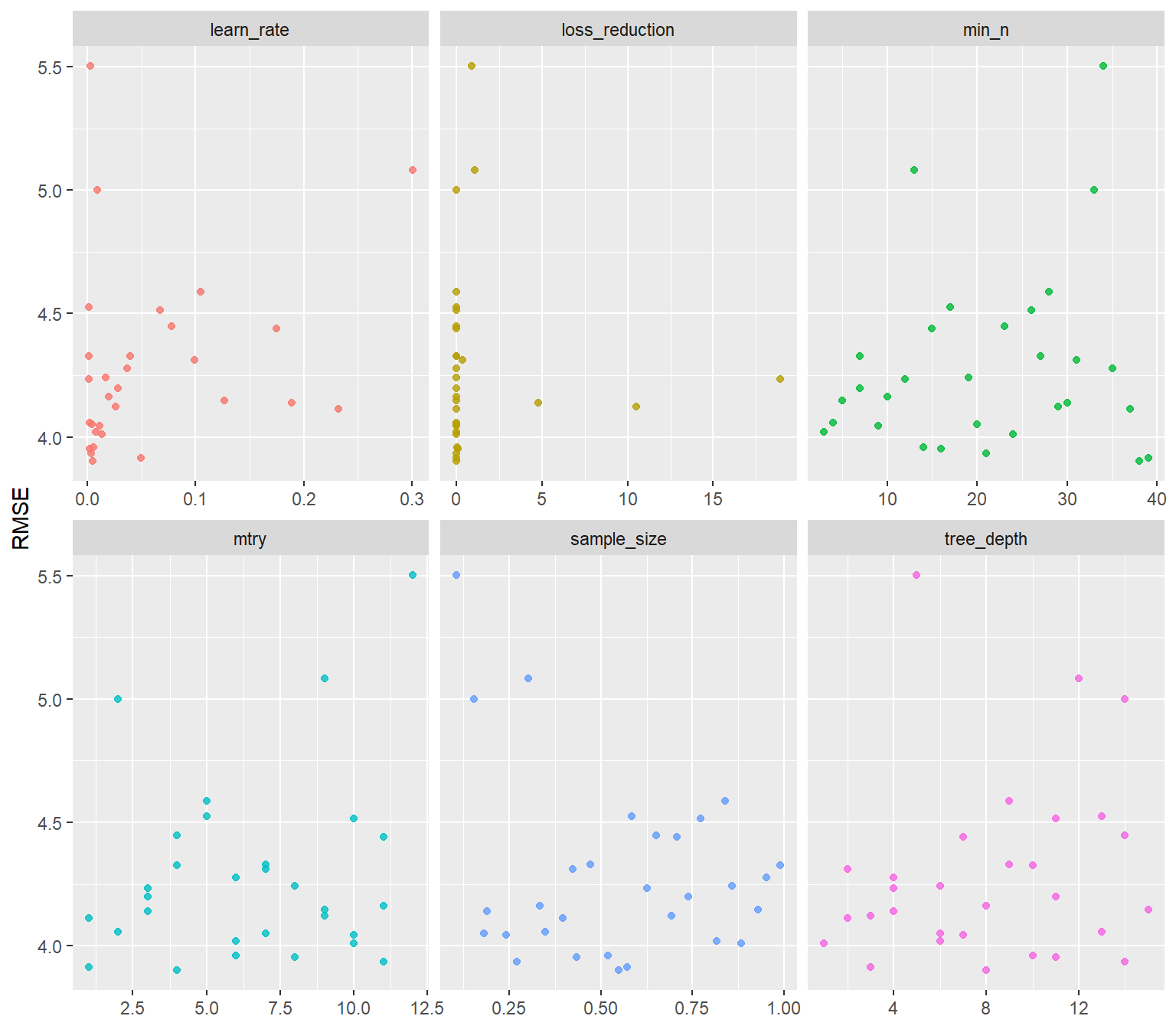

The best XGBoost model

Code

best_rmse <- select_best(xgboost_tune_grid , "rmse")

xgboost_final <- finalize_model(
  xgboost_model,
  best_rmse
)

xgboost_final

Boosted Tree Model Specification (regression)

Main Arguments:
  mtry = 4
  trees = 1000
  min_n = 38
  tree_depth = 8
  learn_rate = 0.00478133186845477
  loss_reduction = 1.00366765721158e-05
  sample_size = 0.548877141447738

Computational engine: xgboost

Fit the model

We can either fit final_tree to training data using fit() or to the testing/training split using last_fit(), which will give us some other results along with the fitted output.

Code

final_fit <- fit(xgboost_final, SOC ~ .,train)

Prediction

Code

test$SOC.pred = predict(final_fit,test)

Code

library(Matrix)
RMSE<- Metrics::rmse(test$SOC, test$SOC.pred$.pred)
RMSE

[1] 3.514375

Code

library(ggpmisc)
formula<-y~x

ggplot(test, aes(SOC,SOC.pred$.pred)) +
  geom_point() +
  geom_smooth(method = "lm")+
  stat_poly_eq(use_label(c("eq", "adj.R2")), formula = formula) +
  ggtitle("XGBoost") +
  xlab("Observed") + ylab("Predicted") +
  scale_x_continuous(limits=c(0,25), breaks=seq(0, 25, 5))+ 
  scale_y_continuous(limits=c(0,25), breaks=seq(0, 25, 5)) +
  # Flip the bars
  theme(
    panel.background = element_rect(fill = "grey95",colour = "gray75",size = 0.5, linetype = "solid"),
    axis.line = element_line(colour = "grey"),
    plot.title = element_text(size = 14, hjust = 0.5),
    axis.title.x = element_text(size = 14),
    axis.title.y = element_text(size = 14),
    axis.text.x=element_text(size=13, colour="black"),
    axis.text.y=element_text(size=13,angle = 90,vjust = 0.5, hjust=0.5, colour='black'))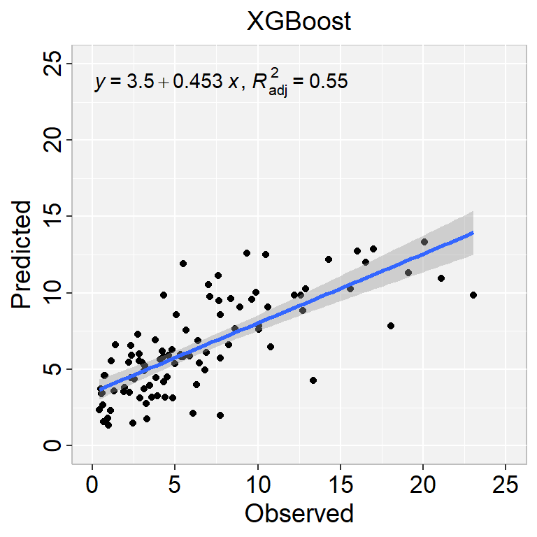

Variable Importance

Code

library(vip)

xgboost_final %>%
  fit( SOC ~ .,train) %>%
  vip(geom = "col")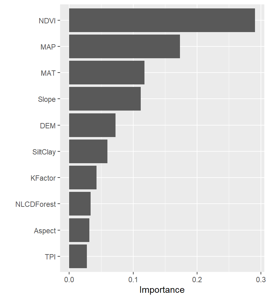

Exercise

Create a R-Markdown documents (name homework_16.rmd) in this project and do all Tasks using the data shown below.
Submit all codes and output as a HTML document (homework_16.html) before class of next week.

Required R-Package

tidyverse, caret, Metrics, tidymodels, vip, bonsai

Data

bd_soil_update.csv

Download the data and save in your project directory. Use read_csv to load the data in your R-session. For example:

mf<-read_csv(“bd_soil_update.csv”)

Tasks

Create a data-frame with following variables for Rajshahi Division:

First use filter() to select data from Rajshai division and then use select() functions to create data-frame with following variables:

SOM, DEM, NDVI, NDFI,

Tune, Fit and show the model performance of a XGBoost model with using tidymodel package

YouTube Video

XGBoost Part 1 (of 4): Regression

Source: StatQuest with Josh Starme

Extreme Gradient Boosting (XGBoost)

Differences between LightGBM vs XGBoost

Extreme Gradient Boosting with “XGBoost” package

Data

Data Preparation

Create training and test dataset

Load the train and test data into the xgboost dataset object

Fit XGBoost model

Prediction

Tunning XGBoost with tidymodel

Data

Split data

Create Recipe

Specify tunable Hypermeters of XGBoost

Create Workflow

Define grid parameters

The best XGBoost model

Fit the model

Prediction

Variable Importance

Exercise

Required R-Package

Data

Tasks

Further Reading

YouTube Video