Introduction to use R

R is an object-oriented programming language like Python, Julia, and JavaScript. Like these programming languages, R has a specific syntax or function, which is essential to understand if you want to use its features to accomplish thousands of things with R. However, one of the most challenging parts of learning R is finding your way around. In section of tutorial you will learn some basic of R such as syntax of R programming, assignment statements, r-data types, control statements and simple r-function.

Screen Prompt

The screen prompt > in R-console is an place to put command or instruction for R to work. Press the “Ctrl” + “L” keys simultaneously. The screen will now be refreshed and the console should be cleared.

R as a Calculator

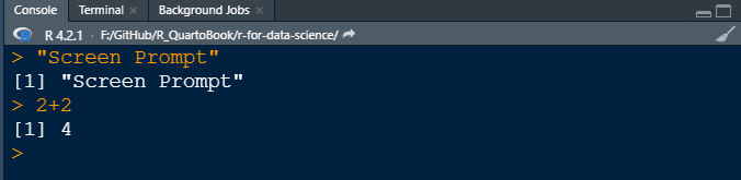
We can use R as a calculators, at the prompt, we enter the expression that we want evaluated and when we hit enter, it will compute the result for us . For Example:

For addition:

Code

2+2

[1] 4

And for subtraction:

Code

4-2

[1] 2

For multiplication:

Code

4*2

[1] 8

For raised to the power:

Code

2^2

[1] 4

Use parentheses to ensure that it understands what you are trying to compute.

https://www.geeksforgeeks.org/control-statements-in-r-programming/?ref=lbp

Syntax of R program

Variables, Comments, and Keywords are the three main components in R- programming. Variables are used to store the data, Comments are used to improve code readability, and Keywords are reserved words that hold a specific meaning to the compiler.

Built in Function

There are so many built-in mathematical functions are available in base-R. Some are shown in below table:

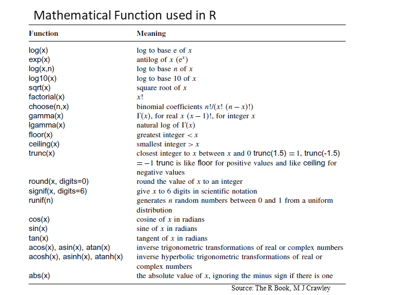
Here below some examples of R built-in R-functions

Code

log10(2)

[1] 0.30103

Code

exp(1)

[1] 2.718282

Code

pi

[1] 3.141593

Code

sin(pi/2)

[1] 1

Number with Exponents

We can use very big numbers or very small numbers in R using the following scheme:

Code

1.2e3 # means 1200 because the e3 means ‘move the decimal point 3 places to the right

[1] 1200

Code

1.2e-2 # means 0.012 because the e-2 means ‘move the decimal point 2 places to the left’

[1] 0.012

Modulo and Integer Quotients

Suppose we want to know the integer part of a division: say, how many 13s are there in 119:

Code

119 %/% 13

[1] 9

Suppose we wanted to know the remainder (what is left over when 119 is divided by 13: in maths this is known as modulo

Code

119 %% 13

[1] 2

Rounding

Several types of rounding (rounding up, rounding down, rounding to the nearest integer) can be done easily with R.

The ‘greatest integer less than’ function is floor()

Code

floor(5.7)

[1] 5

The ‘next integer’ function is ceiling()

Code

ceiling(5.7)

[1] 6

Assignment Statements or assigning values to variables:

Just like in algebra, we often want to store a computation under some variable name. The result is assigned to a variable with the symbols = or <- which is formed by the “less than” symbol followed immediately by a hyphen.

Code

x<-10; # or
y = 12

When you want to know what is in a variable simply ask by typing the variable name.

Code

x; # or

[1] 10

Code

[1] 12

We can store a computation of two variable names and do some calculation and the result is assigned to a new variable

Code

a=2;
b=3;
c=a+b;
c

[1] 5

Variable Names

Do not begin a variable name with a period or a number. Variable names are case (upper/lower) sensitive.
Variable names in R are case-sensitive so x is not the same as X.
Variable names should not begin with numbers (e.g. 1x) or symbols (e.g. %x).
Variable names should not contain blank spaces: use grain.yield

Operators

Code

# + - */%% ^ arithmetic
# > >= < <= == != relational
# ! &  logical
# ~ model formulae
# <- -> assignment
# $ list indexing (the ‘element name’ operator)
# : create a sequence

Basic Data Types

R has a wide variety of data types including scalars, vectors (numerical, character, logical), matrices, data frames, and lists.You can check the type of a variable using the class() function. For example:

Code

x <- 5
class(x) # numeric

[1] "numeric"

Code

y <- "hello"
class(y) # character

[1] "character"

Code

z <- TRUE
class(z) # logical

[1] "logical"

Vectors

A vector is a basic data structure in R that can hold multiple values of the same data type.

A scalar data structure is the most basic data type that holds only a single atomic value at a time. Using scalars, more complex data types can be constructed. The most commonly used scalar types in R:

Numeric
Character or strings
Integer
Logical
Complex

Numeric is the default type used in R for mathematical computations. Examples of numeric are decimal numbers and whole numbers.

Code

x=1.2
x

[1] 1.2

Code

class(x)

[1] "numeric"

Character objects are strings. They could be any sequence of characters including alphabets, numbers, punctuation marks, etc. enclosed in quotes.

Code

Department = 'Chemistry'
School= "University at Buffalo"
class(School)

[1] "character"

Code

paste(Department,",", School)

[1] "Chemistry , University at Buffalo"

Logical values are boolean values of TRUE or FALSE. Note that R needs logical values of TRUE or FALSE to be in upper case. If you use mixed case or lowercase, you’ll get an error or unpredictable results.

Code

u = TRUE; 
v = FALSE
class(u)

[1] "logical"

Code

class(v)

[1] "logical"

A list of numbers or charterers together to form a Multiple Elements Vector. Values can be assigned to vectors in many different ways. We can create a vector of number from 1 to 10, using the concatenation function c

Code

a <- c(1,2,5.3,6,7,8,9,10)
a

[1]  1.0  2.0  5.3  6.0  7.0  8.0  9.0 10.0

Code

s <- c('apple','red',5,TRUE)
print(s)

[1] "apple" "red"   "5"     "TRUE"

It can be generated by the sequence of integer values 1 to 10 using : (colon), the sequence-generating operator,

Code

a<-1:10
a

 [1]  1  2  3  4  5  6  7  8  9 10

We can also create a vector using Using sequence (Seq.) operator.

Code

# Create vector with elements from 5 to 9 incrementing by 0.4.
b = seq(5, 9, by = 0.4)
b

 [1] 5.0 5.4 5.8 6.2 6.6 7.0 7.4 7.8 8.2 8.6 9.0

R has ability to evaluate functions over entire vectors, so no need to write , for loops and subscripts. Important vector functions are listed in below Table:

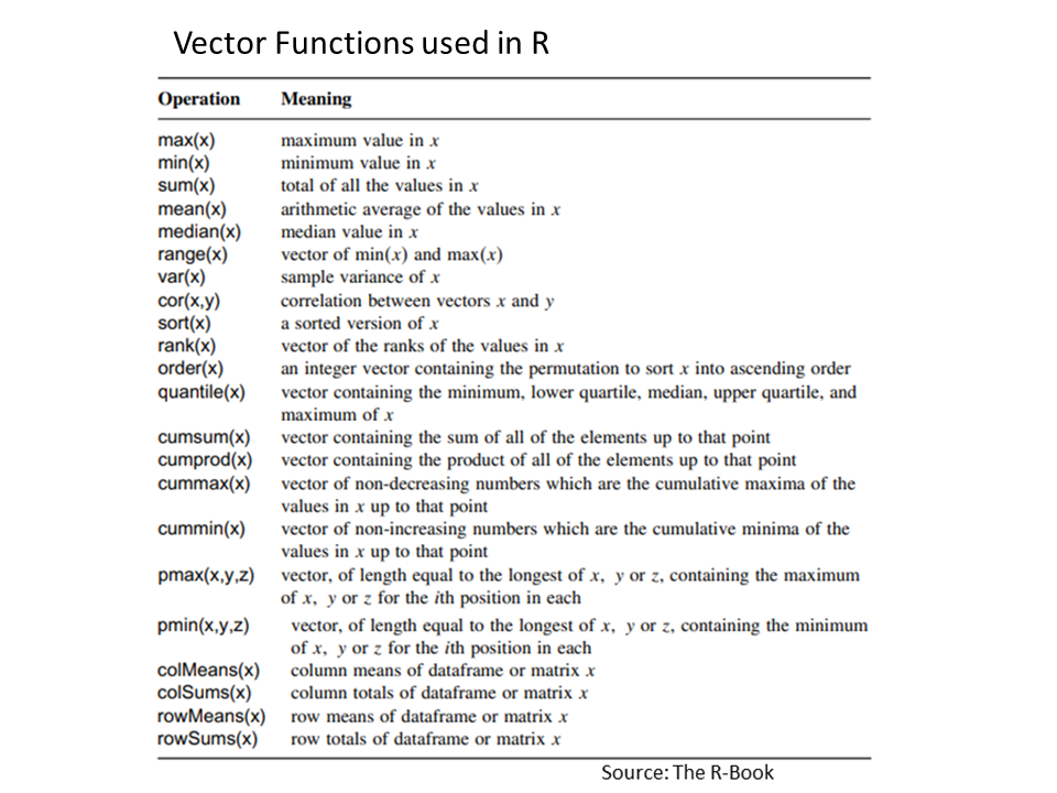
Once we have a vector of numbers we can apply certain built-in functions to them to get useful summaries. For example:

Code

sum(a)        # sums the values in the vector

[1] 55

Code

length(a)     # number of the values in the vector

[1] 10

Code

mean (a)      # the average of the values in the vector

[1] 5.5

Code

var (a)        # the sample variance of the values

[1] 9.166667

Code

sd(a)         # the standard of deviations of the values

[1] 3.02765

Code

max(a)        # the largest value in the vector

[1] 10

Code

min(a)        # the smallest number in the vector

[1] 1

Code

median(a)     # the sample median

[1] 5.5

Summary() function will calculate summary statistics of a vector

Code

summary(a)

   Min. 1st Qu.  Median    Mean 3rd Qu.    Max. 
   1.00    3.25    5.50    5.50    7.75   10.00

Two vectors of same length can be added, subtracted, multiplied or divided giving the result as a vector output.

Code

# Create two vectors.
v1 <- c(3,8,4,5,0,11)
v2 <- c(4,11,0,8,1,2)

Code

# Vector addition.
add.result <- v1+v2
print(add.result)

[1]  7 19  4 13  1 13

Code

# Vector subtraction.
sub.result <- v1-v2
print(sub.result)

[1] -1 -3  4 -3 -1  9

Code

# Vector multiplication.
multi.result <- v1*v2
print(multi.result)

[1] 12 88  0 40  0 22

Code

# Vector division.
divi.result <- v1/v2
print(divi.result)

[1] 0.7500000 0.7272727       Inf 0.6250000 0.0000000 5.5000000

Matrix

Matrices is a two-dimensional rectangular layout of number in rows and columns. All columns in a matrix must have the same mode (numeric, character, etc.) and the same length.

All columns in a matrix must have the same mode (numeric, character, etc.) and the same length. There are several ways of making a matrix. Suppose you were interested in the matrix of 2 x 3. You could form the two rows (vectors) and then bind (rbind) them together to form the matrix:

Code

r1=c(6,2,10)     # row 1
r2=c(1,3,-2)     # row 2
X=rbind(r1,r2)   # binds the vectors into rows a matrix
X

   [,1] [,2] [,3]
r1    6    2   10
r2    1    3   -2

Code

class(X)

[1] "matrix" "array"

We can bind them (cbind) the same vectors into columns of a matrix

Code

Y=cbind(r1,r2)   
Y

     r1 r2
[1,]  6  1
[2,]  2  3
[3,] 10 -2

A Matrix cab be created using the matrix() function from the given set of values. The basic function of a matrix is:

matrix(data, nrow, ncol, byrow, dimnames)

The values are:

data is the input vector which becomes the data elements of the matrix.
nrow is the number of rows to be created.
ncol is the number of columns to be created.
byrow is a logical clue. If TRUE then the input vector elements are arranged by row.
dimname is the names assigned to the rows and columns.

Code

X <- matrix(1:9, nrow = 4, ncol = 3, byrow=T) # row matrix

Warning in matrix(1:9, nrow = 4, ncol = 3, byrow = T): data length [9] is not a
sub-multiple or multiple of the number of rows [4]

Code

     [,1] [,2] [,3]
[1,]    1    2    3
[2,]    4    5    6
[3,]    7    8    9
[4,]    1    2    3

Code

class(X)

[1] "matrix" "array"

Code

attributes(X)

$dim
[1] 4 3

The class and attributes of X indicate that it is a matrix of four rows and three columns (these are its dim attributes)

We can create matrix with row and column names:

Code

# create a vector 
cells=c(1,26,24,68,35,68,73,18,2,56,4,5,34,21,24,20)  # create a vector
# names of column rows
cnames = c("C1","C2","C3","C4") 
# names of two rows
rnames = c("R1","R2","R3","R4") 
# matrix
Z= matrix(cells,nrow=4, ncol=4, byrow=TRUE,dimnames=list(rnames,cnames))
Z

   C1 C2 C3 C4
R1  1 26 24 68
R2 35 68 73 18
R3  2 56  4  5
R4 34 21 24 20

Or, we can easily naming the rows and columns of matrices. Suppose we want to labels rows with Trial names, like Trial.1, Trial.2 etc.:

Code

rownames(X)<-rownames(X, do.NULL=FALSE, prefix="Trial.")
X

        [,1] [,2] [,3]
Trial.1    1    2    3
Trial.2    4    5    6
Trial.3    7    8    9
Trial.4    1    2    3

For column names, we will create a vector of different names for the three most commonly used drugs used in the trial, and use this to specify the colnames(X):

Code

drug.names<-c("Aspirin", "Acetaminophen", "Ibuprofen")
colnames(X)<-drug.names
X

        Aspirin Acetaminophen Ibuprofen
Trial.1       1             2         3
Trial.2       4             5         6
Trial.3       7             8         9
Trial.4       1             2         3

We can access elements of a matrix using the square bracket [] indexing method. Elements can be accessed as var[row, column]. Here rows and columns are vectors.

Code

X[,2]  # 2nd column of a matrix

Trial.1 Trial.2 Trial.3 Trial.4 
      2       5       8       2

Code

X[3,]  # 3rd row of a matrix

      Aspirin Acetaminophen     Ibuprofen 
            7             8             9

Code

X[,2:3] # 2nd and 3rd column

        Acetaminophen Ibuprofen
Trial.1             2         3
Trial.2             5         6
Trial.3             8         9
Trial.4             2         3

Code

X[2:4,1:2]     # rows 2,3,4 of columns 1 and 2

        Aspirin Acetaminophen
Trial.2       4             5
Trial.3       7             8
Trial.4       1             2

We can use summary() function to get row and column wise summary statistics of a matrix

Code

# summary statistics of each column
summary(X)

    Aspirin     Acetaminophen    Ibuprofen   
 Min.   :1.00   Min.   :2.00   Min.   :3.00  
 1st Qu.:1.00   1st Qu.:2.00   1st Qu.:3.00  
 Median :2.50   Median :3.50   Median :4.50  
 Mean   :3.25   Mean   :4.25   Mean   :5.25  
 3rd Qu.:4.75   3rd Qu.:5.75   3rd Qu.:6.75  
 Max.   :7.00   Max.   :8.00   Max.   :9.00

Code

# summary statistics and mean of the column 1 of matrix
summary(X[,1])

   Min. 1st Qu.  Median    Mean 3rd Qu.    Max. 
   1.00    1.00    2.50    3.25    4.75    7.00

Code

# mean
mean(X[,1])

[1] 3.25

Calculated over all the rows and the mean & variance of the bottom row (Trial.4)

Code

mean(X[4,])

[1] 2

Code

var(X[4,])

[1] 1

There are some special functions for calculating summary statistics on matrices

Code

# Total
rowSums(X)

Trial.1 Trial.2 Trial.3 Trial.4 
      6      15      24       6

Code

colSums(X)

      Aspirin Acetaminophen     Ibuprofen 
           13            17            21

Code

# Mean
rowMeans(X)

Trial.1 Trial.2 Trial.3 Trial.4 
      2       5       8       2

Code

colMeans(X)

      Aspirin Acetaminophen     Ibuprofen 
         3.25          4.25          5.25

We can also use apply() function to calculate row and column means. Here columns are margin no. 2 (rows are margin no. 1

Code

apply(X,2,mean)

      Aspirin Acetaminophen     Ibuprofen 
         3.25          4.25          5.25

Code

apply(X,1,mean)

Trial.1 Trial.2 Trial.3 Trial.4 
      2       5       8       2

Factors

Factors are data structures that are implemented to categorize the data or represent categorical data and store it on multiple levels.

In R, factor() function create or convert string-vectors to factors:

Code

# string vectors
gender <- c(rep("male",20), rep("female", 30))
# define factors
gender <- factor(gender) # # 1=female, 2=male internally (alphabetically)
# checking the factors
print(is.factor(gender))

[1] TRUE

Code

class(gender) #

[1] "factor"

Code

summary(gender)

female   male 
    30     20

Lists

List is a one-detrimental data element which consist of several objects in a order. The object in a list may be mixed data types or different data types.The list can be a list of vectors, a list of matrices, a list of characters and a list of functions, and so on.

list in R is created with the use of list() function.

Code

my.list <- list(Location="NY", 
                Year = 2021,
                LabExp=X) # Lab experimental data
             

list(my.list)

[[1]]
[[1]]$Location
[1] "NY"

[[1]]$Year
[1] 2021

[[1]]$LabExp
        Aspirin Acetaminophen Ibuprofen
Trial.1       1             2         3
Trial.2       4             5         6
Trial.3       7             8         9
Trial.4       1             2         3

Components of a list can be accessed in similar fashion like matrix or data frame:

Code

my.list["LabExp"]

$LabExp
        Aspirin Acetaminophen Ibuprofen
Trial.1       1             2         3
Trial.2       4             5         6
Trial.3       7             8         9
Trial.4       1             2         3

Code

my.list["FieldData"]

$<NA>
NULL

Data Frames

In R, tabular data are stored as Data Frame which is made up of three principal components, the data, rows, and columns. It is more general than a matrix, in that different columns can have different modes (numeric, character, factor, etc.).

To create a data frame in R use data.frame() command and then pass each of the vectors you have created as arguments to the function

Code

ID = c(1,2,3,4)    # create a vector of ID coloumn 
Landcover = c("Grassland","Forest", "Arable", "Urban") # create a text vector 
Settlement  = c (FALSE, FALSE, FALSE, TRUE) # creates a logical vector
pH   = c(6.6,4.5, 6.8, 7.5)   # create a numerical vector
SOC  = c (1.2, 3.4, 1.1, 0.12) # create a numerical vector
my.df=data.frame(ID,Landcover,Settlement, pH, SOC) # create a data frame

my.df

  ID Landcover Settlement  pH  SOC
1  1 Grassland      FALSE 6.6 1.20
2  2    Forest      FALSE 4.5 3.40
3  3    Arable      FALSE 6.8 1.10
4  4     Urban       TRUE 7.5 0.12

we can see the detail of structure using str() function

Code

str(my.df)

'data.frame':   4 obs. of  5 variables:
 $ ID        : num  1 2 3 4
 $ Landcover : chr  "Grassland" "Forest" "Arable" "Urban"
 $ Settlement: logi  FALSE FALSE FALSE TRUE
 $ pH        : num  6.6 4.5 6.8 7.5
 $ SOC       : num  1.2 3.4 1.1 0.12

Code

head(my.df)

  ID Landcover Settlement  pH  SOC
1  1 Grassland      FALSE 6.6 1.20
2  2    Forest      FALSE 4.5 3.40
3  3    Arable      FALSE 6.8 1.10
4  4     Urban       TRUE 7.5 0.12

Code

summary(my.df$pH)

   Min. 1st Qu.  Median    Mean 3rd Qu.    Max. 
  4.500   6.075   6.700   6.350   6.975   7.500

Code

summary(my.df[,4:5])

       pH             SOC       
 Min.   :4.500   Min.   :0.120  
 1st Qu.:6.075   1st Qu.:0.855  
 Median :6.700   Median :1.150  
 Mean   :6.350   Mean   :1.455  
 3rd Qu.:6.975   3rd Qu.:1.750  
 Max.   :7.500   Max.   :3.400

Components of data frame can be accessed like a list or like a matrix.

Code

my.df["Landcover"]

  Landcover
1 Grassland
2    Forest
3    Arable
4     Urban

Code

my.df[[2]]

[1] "Grassland" "Forest"    "Arable"    "Urban"

Code

my.df[,4:5]

   pH  SOC
1 6.6 1.20
2 4.5 3.40
3 6.8 1.10
4 7.5 0.12

Control Statements

Control statements are programming language constructs that allow the programmer to control the flow of execution of a program. They are used to alter the order in which statements are executed, and to make decisions based on conditions.

The eight major types of control statements are follows:

if: statement for conditional programming
if..else: statement for conditional programming
for: loop to iterate over a fixed number of iterations
while: loop to iterate until a logical statement returns FALSE
repeat: loop to execute until told to break
break/next:break/next arguments to exit and skip interations in a loop

if Statement

If the expression is true, the statement gets executed. But if the expression is FALSE, nothing happens.

Code

x <- 12
# condition
if(x > 10){
print(paste(x, "is greater than 10"))
}

[1] "12 is greater than 10"

if-else Condition

It is similar to if condition but when the test expression in if condition fails, then statements in else condition are executed.

Code

x <- c(3, 3, -2, 1)

if(any(x < 0)){
        print("x contains negative numbers")
} else{
        print("x contains all positive numbers")
}

[1] "x contains negative numbers"

Code

x <- c(3, 3, 3, 1)

if(any(x < 0)){
        print("x contains negative numbers")
} else{
        print("x contains all positive numbers")
}

[1] "x contains all positive numbers"

for loop

The for loop is used to execute repetitive code statements for a particular number of time. It is useful to iterate over the elements of a list, dataframe, vector, matrix, or any other object.

Code

for (i in 10:15){
        output <- paste("The number is", i)
        print(output)
}

[1] "The number is 10"
[1] "The number is 11"
[1] "The number is 12"
[1] "The number is 13"
[1] "The number is 14"
[1] "The number is 15"

Code

# for loop with vector
x <- c(-8, 3, 12, 15)
for (i in x)
{
    print(i)
}

[1] -8
[1] 3
[1] 12
[1] 15

while loop

While loop executes the same code again and again until a stop condition is met

Code

result <- 1
i <- 1
# test expression
while (i < 5) {
    print(result)
# update expression
   i = i + 1
   result = result + 1
}

[1] 1
[1] 2
[1] 3
[1] 4

Following example show the while statement with break

Code

result <- 1
i <- 1
# test expression
while (i < 5) {
    print(result)
# add break after 2 element 
  if (i==2){
    break
  }
# update expression
   i = i + 1
   result = result + 1
}

[1] 1
[1] 2

Writing R Functions

Writing custom functions is an important part of programming in R.

To create a new R function we need to think about 4 major things:

the name of the function
the arguments (inputs) the function will take
the code the function will run
the output the function will return for the user

To create a function, use the function() keyword:

Code

# create a function with the name my_function
my_function <- function() { 
  print("Hello World!")
}
# call the function
my_function()

[1] "Hello World!"

Arguments are specified after the function name, inside the parentheses. The following example has a function (full_name) with one arguments (last_name). When the function is called, we pass along a first name, which is used inside the function to print the full name:

Code

fulll_name <- function(last_name) {
  paste("Zia",  last_name)
}
fulll_name("Ahmed")

[1] "Zia Ahmed"

To return the results of a function, use the return() function:

Code

addition <- function(x) {
  return (1 + x)
}
print(addition(2))

[1] 3

Code

print(addition(3))

[1] 4

We can create a simple equation with two arguments (x, y):

Code

equation <- function(x, y) {
  a <- x + y
  return(a)
}
equation(2,2)

[1] 4

We can Call a function within another function:

Code

equation(equation(2,4), equation(3,3))

[1] 12

The output above function is therefore (2+4) + (3+3) = 12.

We can also write a function within a function:

Code

x <- 10 
y<- function() {
        r <- 2
        n <- 5
        z <- function() {
                (1+r)^n
        }
        x/z()
}
y()

[1] 0.04115226

Returning Multiple Outputs from a Function:

Code

results_all <- function(x, y) {
        results1 <- 2*x + y
        results2 <- x + 2*y
        results3 <- 2*x + 2*y
        results4 <- x/y
        c(results1, results2, results3, results4)
}
results_all(1, 2)

[1] 4.0 5.0 6.0 0.5

Following function shows an example to convert temperature from Celsius (C) to Fahrenheit (F):

Code

C_to_F = function(C) {
 f = (9/5) * C + 32; # formula
 return(f); # return to
}
C_to_F(10)

[1] 50

Code

C= c(4:10)
C_to_F(C)

[1] 39.2 41.0 42.8 44.6 46.4 48.2 50.0

Apply Family

The apply family consists of vectorized functions which minimize our need to explicitly create loops. These family is an inbuilt R package, so no need to install any packages for the execution.

apply() for matrices and data frames
lapply() for lists…output as list
sapply() for lists…output simplified
tapply() for vectors
mapply() for multi-variant

apply

apply() returns a vector or array or list of values obtained by applying a function to margins of an array or matrix or dataframe. Using apply() is not faster than using a loop function, but it is highly compact and can be written in one line.

apply(x,MARGIN, FUN,…)

Where:

x is the matrix, dataframe or array
MARGIN is a vector giving the subscripts which the function will be applied over. E.g., for a matrix 1 indicates rows, 2 indicates columns, c(1, 2) indicates rows and columns.
FUN is the function to be applied
… is for any other arguments to be passed to the function

Code

# Crate a dataframe
df <- cbind(x1 = 1:8, x2 = 2:9, x3=3:10)
# add row names
dimnames(df)[[1]] <- letters[1:8]

Let’s calculate column mean:

Code

apply(df, 2, mean, trim = 0.2)

 x1  x2  x3 
4.5 5.5 6.5

Row mean:

Code

apply(df, 1, mean, trim = .2)

a b c d e f g h 
2 3 4 5 6 7 8 9

Get column quantile:

Code

apply(df, 2, quantile, probs = c(0.10, 0.25, 0.50, 0.75, 0.90))

      x1   x2   x3
10% 1.70 2.70 3.70
25% 2.75 3.75 4.75
50% 4.50 5.50 6.50
75% 6.25 7.25 8.25
90% 7.30 8.30 9.30

lapply

lapply() returns a list of the same length as X (list), each element of which is the result of applying FUN to the corresponding element of X. It loops over a list, iterating over each element in that list and then applies a function to each element of the list and finally returns a list (l stand for list).

lapply(x, FUN, …)

Where:

x is the list
FUN is the function to be applied
… is for any other arguments to be passed to the function

Code

# Create a list
mylist<-list(A=matrix(1:9,nrow=3),B=1:5,C=c(8,5),  logic = c(TRUE,FALSE,FALSE,TRUE, TRUE))
mylist

$A
     [,1] [,2] [,3]
[1,]    1    4    7
[2,]    2    5    8
[3,]    3    6    9

$B
[1] 1 2 3 4 5

$C
[1] 8 5

$logic
[1]  TRUE FALSE FALSE  TRUE  TRUE

Code

lapply(mylist, mean)

$A
[1] 5

$B
[1] 3

$C
[1] 6.5

$logic
[1] 0.6

You can see how the results are saved as a list form. We can easily unlist the results:

Code

unlist(lapply(mylist,mean))

    A     B     C logic 
  5.0   3.0   6.5   0.6

sapply

sapply() is a wrapper of lapply() to simplify the result to vector or matrix.

Code

sapply(mylist, mean)

    A     B     C logic 
  5.0   3.0   6.5   0.6

tapply

tapply() is used to apply a function over subsets of a vector when a dataset can be broken up into groups (via categorical variables - aka factors)

Code

my.df

  ID Landcover Settlement  pH  SOC
1  1 Grassland      FALSE 6.6 1.20
2  2    Forest      FALSE 4.5 3.40
3  3    Arable      FALSE 6.8 1.10
4  4     Urban       TRUE 7.5 0.12

We can use tapply() to calculate mean values of pH an SOC for land cover

Code

apply(my.df[4:5], 2, function(x) tapply(x, my.df$Landcover, mean))

           pH  SOC
Arable    6.8 1.10
Forest    4.5 3.40
Grassland 6.6 1.20
Urban     7.5 0.12

mapply

mapply() is a multivariate version of sapply(). mapply() applies FUN to the first elements of each … argument, the second elements, the third elements, and so on.

Code

list( rep(2, 4), rep(3, 3), rep(4, 2))

[[1]]
[1] 2 2 2 2

[[2]]
[1] 3 3 3

[[3]]
[1] 4 4

You can see that the same function (rep) is being called repeatedly where the first argument (number vector) varies from 2 to 4, and the second argument (rep) varies from 4 to 2. Instead, you can use mapply()

Code

mapply(rep, 2:4, 4:2)

[[1]]
[1] 2 2 2 2

[[2]]
[1] 3 3 3

[[3]]
[1] 4 4

Introduction to use R

Screen Prompt

R as a Calculator

Syntax of R program

Built in Function

Number with Exponents

Modulo and Integer Quotients

Rounding

Assignment Statements or assigning values to variables:

Variable Names

Operators

Basic Data Types

Vectors

Matrix

Factors

Lists

Data Frames

Control Statements

if Statement

if-else Condition

for loop

while loop

Writing R Functions

Apply Family

apply

lapply

sapply

tapply

mapply

Further Reading