A regression tree is a decision tree used for predicting continuous numerical values rather than categorical ones. Like a decision tree, a regression tree consists of nodes that represent tests on input features. These branches represent possible outcomes of these tests, and leaf nodes that represent final predictions.
The tree is constructed by recursively splitting the data into subsets based on the most informative feature or attribute until a stopping criterion is met. At each split, the goal is to minimize the variance of the target variable within each subset. This is typically done by finding the split that results in the most significant reduction in variance. Once the tree is constructed, it can be used to make predictions by following the path from the root node to a leaf node that corresponds to the input features. The prediction is then the mean or median of the target values of the training examples that belong to the leaf node.
Here are the steps involved in building a regression tree:
Select a split point: Select a feature that will best split the data into two groups. The goal is to minimize the variance of each group. At each node, the algorithm selects a split point for one of the input variables that divides the data into two subsets, such that the variance of the target variable is minimized within each subset.
Calculate the split criteria: A split criteria is calculated to determine the quality of the split. The most commonly used split criteria is the mean squared error (MSE) or the sum of squared errors (SSE).
Repeat for each subset (step 1 and 2): The algorithm then recursively repeats this process on each subset until a stopping criterion is met. This stopping criterion could be a maximum tree depth or a minimum number of data points in a node.
Prediction: Once the tree is built, the prediction is made by traversing the tree from the root node to a leaf node, which corresponds to a final prediction. The prediction is the mean or median value of the target variable within the leaf node.
Regression trees have the advantage of being easy to interpret and visualize, and they can handle both categorical and continuous input features. However, they can be prone to overfitting the training data, especially if the tree becomes too deep. Techniques such as pruning and setting a minimum number of examples per leaf node can be used to prevent overfitting.
The rpart package is an R package for building classification and regression trees using the Recursive Partitioning And Regression Trees (RPART) algorithm. This algorithm uses a top-down, greedy approach to recursively partition the data into smaller subsets, where each subset is homogeneous with respect to the target variable.
The rpart package provides functions for fitting and predicting with regression trees, as well as for visualizing the resulting tree. Some of the main functions in the rpart package include:
rpart(): This function is used to fit a regression or classification tree to the data. It takes a formula, a data frame, and optional arguments for controlling the tree-building process.
predict.rpart(): This function is used to predict the target variable for new data using a fitted regression or classification tree.
printcp(): This function is used to print the complexity parameter table for a fitted regression or classification tree. This table shows the cross-validated error rate for different values of the complexity parameter, which controls the size of the tree.
plot(): This function is used to visualize a fitted regression or classification tree. It produces a graphical representation of the tree with the nodes and branches labeled.
install.package(“rpart”)
install.package(“rpart.plot”)
Code
library(rpart) #for fitting decision treeslibrary(rpart.plot) #for plotting decision trees
The rpart() function takes as input a formula specifying the target variable to be predicted and the predictors to be used in the model, as well as a data set containing the observations. It then recursively partitions the data based on the predictors, creating a tree structure in which each internal node represents a decision based on a predictor and each leaf node represents a predicted value for the target variable.
First, we’ll build a large initial regression tree. We can ensure that the tree is large by using a small value for cp, which stands for “complexity parameter.”
We’ll then use the printcp() function to print the results of the model:
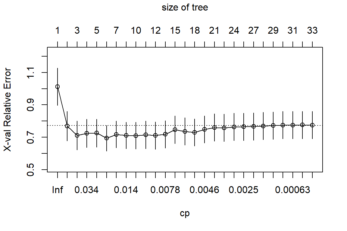
We can use the plotcp() function to visualize the cross-validated error for each level of tree complexity:
Code
plotcp(in.fit)
Prune the tree
Pruning is a technique used to reduce the size of a regression tree by removing some of the branches that do not contribute much to the prediction accuracy. Pruning can help to avoid overfitting and improve the generalization performance of the model.
Next, we’ll prune the regression tree to find the optimal value to use for cp (the complexity parameter) that leads to the lowest test error. Use the prune() function to prune the tree to the desired complexity level. For example, to prune the tree to the level with the lowest cross-validated error.
Note that the optimal value for cp is the one that leads to the lowest xerror in the previous output, which represents the error on the observations from the cross-validation data.
CART

371 samples
  8 predictor

No pre-processing
Resampling: Cross-Validated (10 fold, repeated 5 times)
Summary of sample sizes: 334, 333, 334, 334, 334, 334, ...
Resampling results across tuning parameters:

  cp    RMSE      Rsquared      MAE
  0.00  4.509316  2.769299e-01  3.231612
  0.01  4.323208  3.072242e-01  3.032395
  0.02  4.257813  3.158449e-01  2.998006
  0.03  4.314825  2.956942e-01  3.049286
  0.04  4.294635  2.931849e-01  3.022898
  0.05  4.253645  3.052001e-01  3.017513
  0.06  4.201570  3.150752e-01  3.011249
  0.07  4.173444  3.175855e-01  3.004081
  0.08  4.222658  3.033084e-01  3.043568
  0.09  4.388515  2.488704e-01  3.191270
  0.10  4.405598  2.423928e-01  3.243067
  0.11  4.405598  2.423928e-01  3.243067
  0.12  4.405598  2.423928e-01  3.243067
  0.13  4.405598  2.423928e-01  3.243067
  0.14  4.405598  2.423928e-01  3.243067
  0.15  4.405598  2.423928e-01  3.243067
  0.16  4.405598  2.423928e-01  3.243067
  0.17  4.405598  2.423928e-01  3.243067
  0.18  4.405598  2.423928e-01  3.243067
  0.19  4.405598  2.423928e-01  3.243067
  0.20  4.405598  2.423928e-01  3.243067
  0.21  4.405598  2.423928e-01  3.243067
  0.22  4.405598  2.423928e-01  3.243067
  0.23  4.459716  2.308527e-01  3.287461
  0.24  4.480471  2.278248e-01  3.300437
  0.25  4.646920  1.945108e-01  3.441228
  0.26  4.796143  1.580023e-01  3.587896
  0.27  4.921510  1.206834e-01  3.721628
  0.28  4.960463  7.138244e-02  3.760534
  0.29  4.969457  1.861139e-05  3.789281
  0.30  4.960423           NaN  3.787247
  0.31  4.960423           NaN  3.787247
  0.32  4.960423           NaN  3.787247
  0.33  4.960423           NaN  3.787247
  0.34  4.960423           NaN  3.787247
  0.35  4.960423           NaN  3.787247
  0.36  4.960423           NaN  3.787247
  0.37  4.960423           NaN  3.787247
  0.38  4.960423           NaN  3.787247
  0.39  4.960423           NaN  3.787247
  0.40  4.960423           NaN  3.787247

RMSE was used to select the optimal model using the smallest value.
The final value used for the model was cp = 0.07.
Code
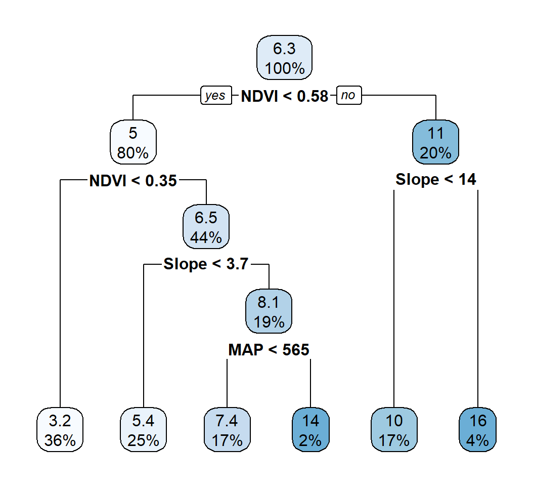
rpart.plot(train.rpart$finalModel)
Regression Tree with tidymodel
The tidymodels provides a comprehensive framework for building, tuning, and fit regression tree models while following the principles of the tidyverse.
Split data
Code
library(tidymodels)set.seed(1245) # for reproducibilitysplit <-initial_split(df, prop =0.8, strata = SOC)train <- split %>%training()test <- split %>%testing()# Set 10 fold cross-validation data set cv_folds <-vfold_cv(train, v =10)
Create Recipe
A recipe is a description of the steps to be applied to a data set in order to prepare it for data analysis. Before training the model, we can use a recipe to do some preprocessing required by the model.
Code
# load librarylibrary(tidymodels)# Create a recipetree_recipe <-recipe(SOC ~ ., data = train) %>%step_zv(all_predictors()) %>%step_dummy(all_nominal()) %>%step_normalize(all_numeric_predictors())
Specify tunable decision tree model
decision_tree() from parsnip package (installed with tidymodels) defines a model as a set of if/then statements that creates a tree-based structure. This function can fit classification, regression, and censored regression models. We will use rpart to create a regression tree model
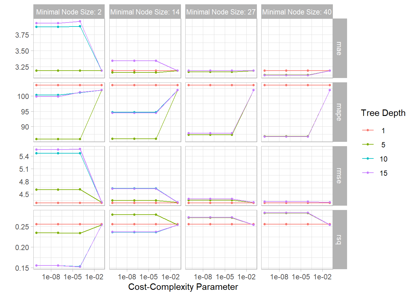
Now we will fit the models with all the possible parameter values on all our resampled (cv.fold) datasets. tune_grid() of tune package (installed with tidymodels) computes a set of performance metrics (e.g. accuracy or RMSE) for a pre-defined set of tuning parameters that correspond to a model or recipe across one or more resamples of the data.
tune_grid() computes a set of performance metrics (e.g. accuracy or RMSE) for a pre-defined set of tuning parameters that correspond to a model or recipe across one or more resamples of the data.
We will use registerDoParallel() function that register the parallel backend with the foreach package.
Decision Tree Model Specification (regression)

Main Arguments:
  cost_complexity = 1e-10
  tree_depth = 1
  min_n = 2

Computational engine: rpart
We can either fit final_tree to training data using fit() or to the testing/training split using last_fit(), which will give us some other results along with the fitted output.
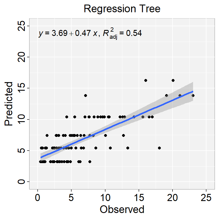
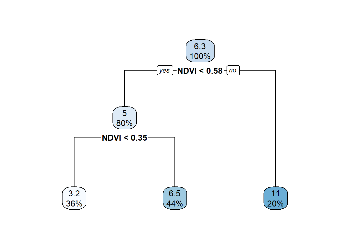
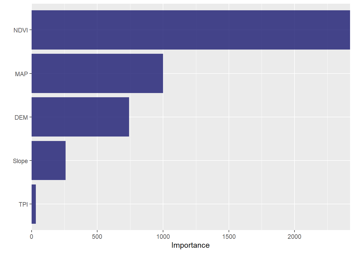
[{fig-align="right" width="176" height="64"}](https://github.com/zia207/r-colab/blob/main/regression_tree.ipynb)# Regression Trees {.unnumbered}A regression tree is a decision tree used for predicting continuous numerical values rather than categorical ones. Like a decision tree, a regression tree consists of nodes that represent tests on input features. These branches represent possible outcomes of these tests, and leaf nodes that represent final predictions.The tree is constructed by recursively splitting the data into subsets based on the most informative feature or attribute until a stopping criterion is met. At each split, the goal is to minimize the variance of the target variable within each subset. This is typically done by finding the split that results in the most significant reduction in variance. Once the tree is constructed, it can be used to make predictions by following the path from the root node to a leaf node that corresponds to the input features. The prediction is then the mean or median of the target values of the training examples that belong to the leaf node.Here are the steps involved in building a regression tree:1. Select a split point: Select a feature that will best split the data into two groups. The goal is to minimize the variance of each group. At each node, the algorithm selects a split point for one of the input variables that divides the data into two subsets, such that the variance of the target variable is minimized within each subset.2. Calculate the split criteria: A split criteria is calculated to determine the quality of the split. The most commonly used split criteria is the mean squared error (MSE) or the sum of squared errors (SSE).3. Repeat for each subset (step 1 and 2): The algorithm then recursively repeats this process on each subset until a stopping criterion is met. This stopping criterion could be a maximum tree depth or a minimum number of data points in a node.4. Prediction: Once the tree is built, the prediction is made by traversing the tree from the root node to a leaf node, which corresponds to a final prediction. The prediction is the mean or median value of the target variable within the leaf node.Regression trees have the advantage of being easy to interpret and visualize, and they can handle both categorical and continuous input features. However, they can be prone to overfitting the training data, especially if the tree becomes too deep. Techniques such as pruning and setting a minimum number of examples per leaf node can be used to prevent overfitting.### DataIn this exercise, we will use following data set.[gp_soil_data.csv](https://www.dropbox.com/s/9ikm5yct36oflei/gp_soil_data.csv?dl=0)```{r}#| warning: false#| error: falselibrary(tidyverse)# define file from my githuburlfile ="https://github.com//zia207/r-colab/raw/main/Data/USA/gp_soil_data.csv"mf<-read_csv(url(urlfile))# Create a data-framedf<-mf %>% dplyr::select(SOC, DEM, Slope, TPI,MAT, MAP,NDVI, NLCD, FRG)%>%glimpse()```## Regression tree with rpartThe rpart package is an R package for building classification and regression trees using the Recursive Partitioning And Regression Trees (RPART) algorithm. This algorithm uses a top-down, greedy approach to recursively partition the data into smaller subsets, where each subset is homogeneous with respect to the target variable.The rpart package provides functions for fitting and predicting with regression trees, as well as for visualizing the resulting tree. Some of the main functions in the rpart package include:rpart(): This function is used to fit a regression or classification tree to the data. It takes a formula, a data frame, and optional arguments for controlling the tree-building process.predict.rpart(): This function is used to predict the target variable for new data using a fitted regression or classification tree.printcp(): This function is used to print the complexity parameter table for a fitted regression or classification tree. This table shows the cross-validated error rate for different values of the complexity parameter, which controls the size of the tree.plot(): This function is used to visualize a fitted regression or classification tree. It produces a graphical representation of the tree with the nodes and branches labeled.> install.package("rpart")> install.package("rpart.plot")```{r}#| warning: false#| error: falselibrary(rpart) #for fitting decision treeslibrary(rpart.plot) #for plotting decision trees```### Split the data```{r}#| warning: false#| error: falselibrary(tidymodels)set.seed(1245) # for reproducibilitysplit.df <-initial_split(df, prop =0.8, strata = SOC)train.df <- split.df %>%training()test.df <- split.df %>%testing()```### Build the initial regression treeThe rpart() function takes as input a formula specifying the target variable to be predicted and the predictors to be used in the model, as well as a data set containing the observations. It then recursively partitions the data based on the predictors, creating a tree structure in which each internal node represents a decision based on a predictor and each leaf node represents a predicted value for the target variable.First, we'll build a large initial regression tree. We can ensure that the tree is large by using a small value for cp, which stands for "complexity parameter."We'll then use the printcp() function to print the results of the model:```{r}#| warning: false#| error: falsein.fit <-rpart(SOC ~ ., data=train.df, control=rpart.control(cp=.0001),method ="anova")#view resultsprintcp(in.fit)```We can use the plotcp() function to visualize the cross-validated error for each level of tree complexity:```{r}#| warning: false#| error: false#| fig.width: 6#| fig.height: 4plotcp(in.fit)```### Prune the treePruning is a technique used to reduce the size of a regression tree by removing some of the branches that do not contribute much to the prediction accuracy. Pruning can help to avoid overfitting and improve the generalization performance of the model.Next, we'll prune the regression tree to find the optimal value to use for cp (the complexity parameter) that leads to the lowest test error. Use the prune() function to prune the tree to the desired complexity level. For example, to prune the tree to the level with the lowest cross-validated error.Note that the optimal value for cp is the one that leads to the lowest xerror in the previous output, which represents the error on the observations from the cross-validation data.First, #identify best cp value to use:```{r}#| warning: false#| error: falsebest_cp <-in.fit$cptable[which.min(in.fit$cptable[,"xerror"]),"CP"]best_cp```We use use this cp value to prune the tree:```{r}#| warning: false#| error: falsepruned.fit <- rpart::prune(in.fit, cp = best_cp)summary(pruned.fit)```We can use rpart.plot() function to plot the regression tree:```{r}#| warning: false#| error: false#| fig.width: 5.5#| fig.height: 5rpart.plot(pruned.fit)```### Prediction```{r}#| warning: false#| error: falsetest.df$SOC.tree<-predict(pruned.fit, test.df)``````{r}#| warning: false#| error: falseRMSE<- Metrics::rmse(test.df$SOC, test.df$SOC.tree)RMSE``````{r}#| warning: false#| error: false#| fig.width: 4#| fig.height: 4library(ggpmisc)formula<-y~xggplot(test.df, aes(SOC,SOC.tree)) +geom_point() +geom_smooth(method ="lm")+stat_poly_eq(use_label(c("eq", "adj.R2")), formula = formula) +ggtitle("Regression Tree") +xlab("Observed") +ylab("Predicted") +scale_x_continuous(limits=c(0,25), breaks=seq(0, 25, 5))+scale_y_continuous(limits=c(0,25), breaks=seq(0, 25, 5)) +# Flip the barstheme(panel.background =element_rect(fill ="grey95",colour ="gray75",size =0.5, linetype ="solid"),axis.line =element_line(colour ="grey"),plot.title =element_text(size =14, hjust =0.5),axis.title.x =element_text(size =14),axis.title.y =element_text(size =14),axis.text.x=element_text(size=13, colour="black"),axis.text.y=element_text(size=13,angle =90,vjust =0.5, hjust=0.5, colour='black'))```## Regression Tree with Caret Package### Set control Parameters```{r}#| warning: false#| error: falselibrary(caret)set.seed(123)train.control <-trainControl(method ="repeatedcv", number =10, repeats =5,preProc =c("center", "scale", "nzv"))```### Train the model```{r}#| warning: false#| error: falseset.seed(2)train.rpart <- caret::train(SOC ~., data = train.df,method ="rpart",tuneLength =50,trControl = train.control ,tuneGrid =expand.grid(cp =seq(0,0.4,0.01)))``````{r}train.rpart``````{r}rpart.plot(train.rpart$finalModel)```## Regression Tree with tidymodelThe tidymodels provides a comprehensive framework for building, tuning, and fit regression tree models while following the principles of the tidyverse.### Split data```{r}library(tidymodels)set.seed(1245) # for reproducibilitysplit <-initial_split(df, prop =0.8, strata = SOC)train <- split %>%training()test <- split %>%testing()# Set 10 fold cross-validation data set cv_folds <-vfold_cv(train, v =10)```### Create RecipeA recipe is a description of the steps to be applied to a data set in order to prepare it for data analysis. Before training the model, we can use a recipe to do some preprocessing required by the model.```{r}#| warning: false#| error: false# load librarylibrary(tidymodels)# Create a recipetree_recipe <-recipe(SOC ~ ., data = train) %>%step_zv(all_predictors()) %>%step_dummy(all_nominal()) %>%step_normalize(all_numeric_predictors())```### Specify tunable decision tree modeldecision_tree() from parsnip package (installed with tidymodels) defines a model as a set of if/then statements that creates a tree-based structure. This function can fit classification, regression, and censored regression models. We will use **rpart** to create a regression tree model```{r}#| warning: false#| error: falsetree_model<-decision_tree(cost_complexity =tune(),tree_depth =tune(),min_n =tune()) %>%set_engine("rpart") %>%set_mode("regression")tree_model```### Define workflow```{r}#| warning: false#| error: falsetree_wf <-workflow() %>%add_recipe(tree_recipe) %>%add_model(tree_model)```### Define possible grid parameterWe use grid_regular() function of dials package (installed with tidymodesl) to create grids of tuning parameters```{r}#| warning: false#| error: falsetree_grid <-grid_regular(cost_complexity(), tree_depth(), min_n(), levels =4)head(tree_grid)```### Model tuning via grid searchNow we will fit the models with all the possible parameter values on all our resampled (cv.fold) datasets. tune_grid() of tune package (installed with tidymodels) computes a set of performance metrics (e.g. accuracy or RMSE) for a pre-defined set of tuning parameters that correspond to a model or recipe across one or more resamples of the data.tune_grid() computes a set of performance metrics (e.g. accuracy or RMSE) for a pre-defined set of tuning parameters that correspond to a model or recipe across one or more resamples of the data.We will use registerDoParallel() function that register the parallel backend with the foreach package.> install.pckages("doParallel")```{r}#| warning: false#| error: false## register the parallel backenddoParallel::registerDoParallel()set.seed(345)tree_tune <-tune_grid( tree_wf,resamples = cv_folds,grid = tree_grid,metrics =metric_set(rmse, rsq, mae, mape))tree_tune```### Evaluate modelcollect_metrics() of tune package (installed with tidymodels) obtain and format results by tuneing function:```{r}#| warning: false#| error: falsecollect_metrics(tree_tune)```we can also visualize the tuning parameters:```{r}#| warning: false#| error: falseautoplot(tree_tune) +theme_light(base_family ="IBMPlexSans")```### The best tuning parametersshow_best() of tune package displays the top sub-models and their performance estimates.```{r}#| warning: false#| error: falseshow_best(tree_tune, "rmse")```select_best() finds the tuning parameter combination with the best performance values.```{r}#| warning: false#| error: falseselect_best(tree_tune, "rmse")```### Final tree model```{r}#| warning: false#| error: falsetree_final <-finalize_model(tree_model, select_best(tree_tune, "rmse"))tree_final```We can either fit final_tree to training data using fit() or to the testing/training split using last_fit(), which will give us some other results along with the fitted output.```{r}#| warning: false#| error: falsefinal_fit <-fit(tree_final, SOC ~ .,train)final_reg <-last_fit(tree_final, SOC ~ ., split)``````{r}collect_metrics(final_reg)```### Prediction```{r}predict(final_fit,test)```### Variable importance plotvip() function can plot variable importance scores for the predictors in a model.> imstall.package("vip")```{r}#| warning: false#| error: false#| fig.width: 4.5#| fig.height: 6library(vip)final_fit %>%vip(geom ="col", aesthetics =list(fill ="midnightblue", alpha =0.8)) +scale_y_continuous(expand =c(0, 0))```### Exercise1. Create a R-Markdown documents (name homework_13.rmd) in this project and do all Tasks using the data shown below.2. Submit all codes and output as a HTML document (homework_13.html) before class of next week.#### Required R-Packagetidyverse, caret, Metrics, tidymodels, vip#### Data1. [bd_soil_update.csv](https://www.dropbox.com/s/jtzycm4kg3lngu3/bd_soil_update.csv?dl=0)Download the data and save in your project directory. Use read_csv to load the data in your R-session. For example:> mf\<-read_csv("bd_soil_update.csv")#### Tasks1. Create a data-frame for a regression tree model of SOC with following variables for Rajshahi Division: First use filter() to select data from Rajshai division and then use select() functions to create data-frame with following variables: SOM, DEM, NDVI, NDFI,2. Fit a regression tree model with grid search using, caret, tidymodels and h20 packages3. Show all steps of data processing, grid search, fit model, prediction and VIP### Further Reading1. [Tune and interpret decision trees for #TidyTuesday wind turbines](https://juliasilge.com/blog/wind-turbine/)2. [ISLR8 - Decision Trees in R (Regression)](https://rstudio-pubs-static.s3.amazonaws.com/446972_323b4475ff0749228fe4057c4d7685f5.html)3. https://www.r-bloggers.com/2021/04/decision-trees-in-r/### YouTube Video1. Visual Guide to Regression Trees{{< video https://www.youtube.com/watch?v=g9c66TUylZ4 >}}Source: [StatQuest with Josh Starme](https://www.youtube.com/@statquest)