Data Exploration with dlookr

The dlookr is a collection of tools that support data diagnosis, exploration, and transformation. Data diagnostics provides information and visualization of missing values and outliers and unique and negative values to help you understand the distribution and quality of your data. Data exploration provides information and visualization of the descriptive statistics of univariate variables, normality tests and outliers, correlation of two variables, and relationship between target variable and predictor. Data transformation supports binning for categorizing continuous variables, imputates missing values and outliers, resolving skewness. And it creates automated reports that support these three tasks.

Features:

• Diagnose data quality.

• Find appropriate scenarios to pursuit the follow-up analysis through data exploration and understanding.

• Derive new variables or perform variable transformations.

• Automatically generate reports for the above three tasks.

• Supports quality diagnosis and EDA of table of DBMS

Usage

• Data quality diagnosis for data.frame, tbl_df, and table of DBMS

• Exploratory Data Analysis for data.frame, tbl_df, and table of DBMS

• Data Transformation

• Data diagnosis and EDA for table of DBMS

install.packages("dlookr")

Load Library

Code

library(dlookr)

Data

In this exercise we will use following data set. The data set has missing values.

gp_soil_data_na.csv

Code

library(tidyverse)
# define file from my github
urlfile = "https://github.com/zia207/r-colab/raw/main/Data/USA/gp_soil_data_na.csv"
mf<-read_csv(url(urlfile))

Data Quality Diagnosis

General diagnosis of all variables

Data Quality Diagnosis is the first step before any statistical analysis. We use diagnose() function of dlookr package to do general General diagnosis of all variables.

The variables of the tbl_df object returned by diagnose () are as follows:

• variables : variable names

• types : the data type of the variables

• missing_count : number of missing values

• missing_percent : percentage of missing values

• unique_count : number of unique values

• unique_rate : rate of unique value. unique_count / number of observation

Code

library (flextable)
dlookr::diagnose(mf)%>% 
  flextable() 

variables	types	missing_count	missing_percent	unique_count	unique_rate
ID	numeric	0	0.0000000	471	1.000000000
FIPS	numeric	0	0.0000000	172	0.365180467
STATE_ID	numeric	0	0.0000000	4	0.008492569
STATE	character	0	0.0000000	4	0.008492569
COUNTY	character	0	0.0000000	161	0.341825902
Longitude	numeric	0	0.0000000	471	1.000000000
Latitude	numeric	0	0.0000000	471	1.000000000
SOC	numeric	4	0.8492569	457	0.970276008
DEM	numeric	0	0.0000000	464	0.985138004
Aspect	numeric	0	0.0000000	464	0.985138004
Slope	numeric	0	0.0000000	464	0.985138004
TPI	numeric	0	0.0000000	464	0.985138004
KFactor	numeric	0	0.0000000	386	0.819532909
MAP	numeric	0	0.0000000	464	0.985138004
MAT	numeric	0	0.0000000	463	0.983014862
NDVI	numeric	0	0.0000000	464	0.985138004
SiltClay	numeric	0	0.0000000	462	0.980891720
NLCD	character	0	0.0000000	4	0.008492569
FRG	character	0	0.0000000	6	0.012738854

Missing Value(NA) : Variables with many missing values, i.e. those with a missing_percent close to 100, should be excluded from the analysis.

Unique value : Variables with a unique value (unique_count = 1) are considered to be excluded from data analysis. And if the data type is not numeric (integer, numeric) and the number of unique values is equal to the number of observations (unique_rate = 1), then the variable is likely to be an identifier. Therefore, this variable is also not suitable for the analysis model.

Diagnosis of Numeric Variables

We may use diagnose_numeric(), diagnoses numeric(continuous and discrete) variables in a data frame returns more diagnostic information such as:

• min : minimum value

• Q1 : 1/4 quartile, 25th percentile

• mean : arithmetic mean

• median : median, 50th percentile

• Q3 : 3/4 quartile, 75th percentile

• max : maximum value

• zero : number of observations with a value of 0

• minus : number of observations with negative numbers

• outlier : number of outliers

Code

# First select  numerical columns
mf %>% 
  dplyr::select(SOC, DEM, Slope, Aspect, TPI, KFactor, MAP, MAT, NDVI, SiltClay) %>%
# then diagnose them
  dlookr::diagnose_numeric()%>% 
  flextable()

variables	min	Q1	mean	median	Q3	max	zero	minus	outlier
SOC	0.4080000	2.7695000	6.3507623126	4.97100000	8.7135000	30.4730000	0	0	20
DEM	258.6488037	1,175.3313595	1,631.1063060667	1,592.89318800	2,234.2648930	3,618.0241700	0	0	0
Slope	0.6492527	1.4506671	4.8267398902	2.72667742	7.1070788	26.1041622	0	0	20
Aspect	86.8945694	148.8052292	165.4676589153	164.07072450	179.0842895	255.8335266	0	0	8
TPI	-26.7086506	-0.8160543	-0.0006690991	-0.04758827	0.8490718	16.7062569	0	241	85
KFactor	0.0500000	0.1933357	0.2558965090	0.28000000	0.3200000	0.4300000	0	0	0
MAP	193.9132233	352.7745056	499.3729530231	432.63040160	590.4269104	1,128.1145020	0	0	17
MAT	-0.5910638	5.8800533	8.8855210982	9.17283535	12.4442859	16.8742866	0	6	0
NDVI	0.1424335	0.3053468	0.4354311144	0.41568252	0.5559025	0.7969922	0	0	0
SiltClay	9.1619568	42.7587299	53.6779156034	52.11276627	62.8508625	89.8344116	0	0	3

Diagnosis of Categorical Variables

diagnose_category() diagnoses the categorical(factor, ordered, character) variables of a data frame. The usage is similar to diagnose() but returns more diagnostic information such as:

• variables : variable names

• levels: level names

• N : number of observation

• freq : number of observation at the levels

• ratio : percentage of observation at the levels

• rank : rank of occupancy ratio of levels

Code

mf %>% 
# Select categorical variables
  dplyr::select(STATE, NLCD,FRG) %>%
# then diagnose them
  dlookr::diagnose_category()%>% 
  flextable()

variables	levels	N	freq	ratio	rank
STATE	Colorado	471	136	28.874735	1
STATE	Wyoming	471	120	25.477707	2
STATE	New Mexico	471	109	23.142251	3
STATE	Kansas	471	106	22.505308	4
NLCD	Herbaceous	471	151	32.059448	1
NLCD	Shrubland	471	130	27.600849	2
NLCD	Planted/Cultivated	471	97	20.594480	3
NLCD	Forest	471	93	19.745223	4
FRG	Fire Regime Group II	471	252	53.503185	1
FRG	Fire Regime Group III	471	100	21.231423	2
FRG	Fire Regime Group IV	471	75	15.923567	3
FRG	Fire Regime Group I	471	19	4.033970	4
FRG	Fire Regime Group V	471	18	3.821656	5
FRG	Indeterminate FRG	471	7	1.486200	6

Diagnosing Outliers

diagnose_outlier() diagnoses the outliers of the numeric (continuous and discrete) variables of the data frame.

• outliers_cnt : number of outliers

• outliers_ratio : percent of outliers

• outliers_mean : arithmetic average of outliers

• with_mean : arithmetic average of with outliers

• without_mean : arithmetic average of without outliers

The diagnose_outlier() produces outlier information for diagnosing the quality of the numerical data.

Code

mf %>% dlookr::diagnose_outlier(SOC, DEM, SOC, Slope, Aspect, TPI, KFactor, MAP, MAT, NDVI, SiltClay)

# A tibble: 10 × 6
   variables outliers_cnt outliers_ratio outliers_mean   with_mean without_mean
   <chr>            <int>          <dbl>         <dbl>       <dbl>        <dbl>
 1 SOC                 20          4.25         21.1      6.35           5.69  
 2 DEM                  0          0           NaN     1631.          1631.    
 3 Slope               20          4.25         18.9      4.83           4.20  
 4 Aspect               8          1.70        224.     165.           164.    
 5 TPI                 85         18.0           0.291   -0.000669      -0.0649
 6 KFactor              0          0           NaN        0.256          0.256 
 7 MAP                 17          3.61       1049.     499.           479.    
 8 MAT                  0          0           NaN        8.89           8.89  
 9 NDVI                 0          0           NaN        0.435          0.435 
10 SiltClay             3          0.637         9.71    53.7           54.0   

Visualization of Outliers

plot_outlier() visualizes outliers of numerical variables(continuous and discrete) of data.frame. Usage is the same diagnose().

The plot derived from the numerical data diagnosis is as follows.

• With outliers box plot

• Without outliers box plot

• With outliers histogram

• Without outliers histogram

The following example uses plot_outlier() after diagnose_outlier, and filter and select with dplyr packages to visualize this with an outlier ratio of 0.5% or higher.

Code

mf %>%
  dlookr::plot_outlier(dlookr::diagnose_outlier(mf,SOC) %>% 
                 dplyr::filter(outliers_ratio >= 0.5) %>% 
                 dplyr::select(variables) %>% 
                 unlist())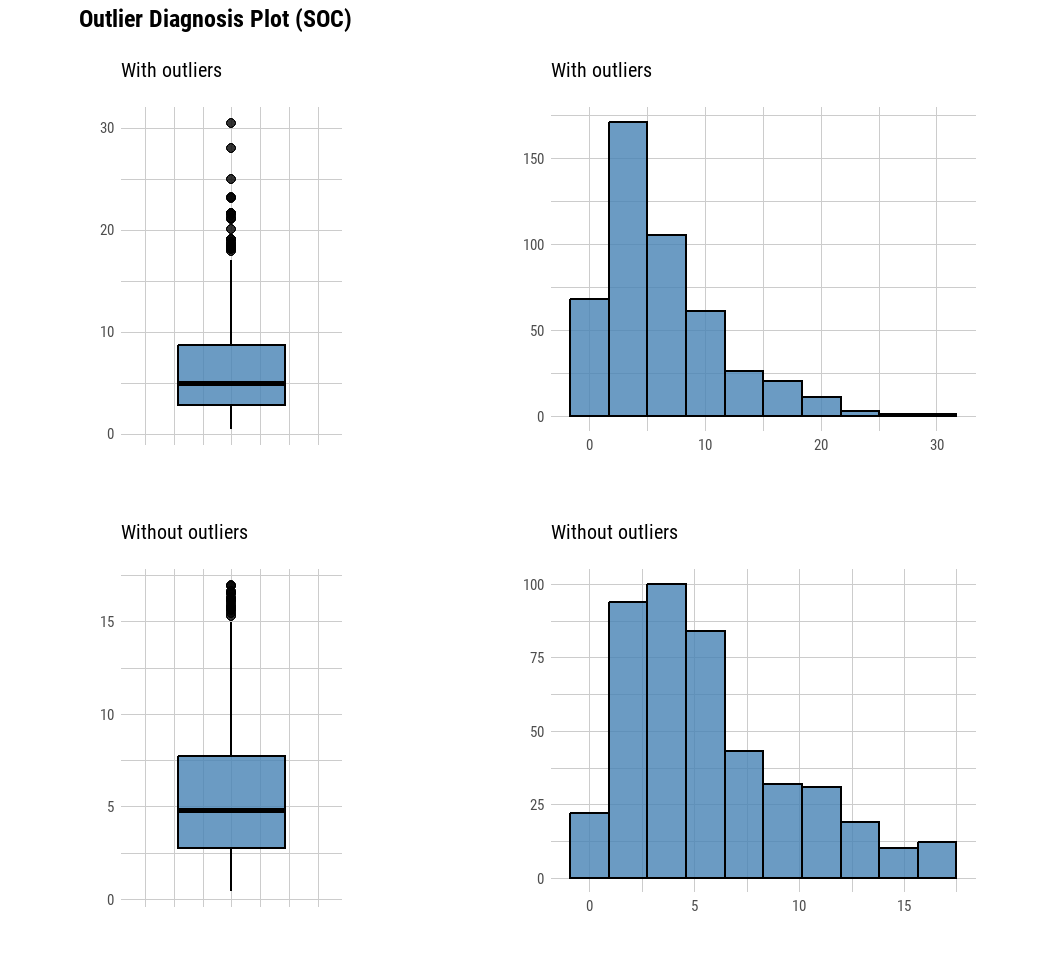

Daignosis Normality

Normality Test

normality() function of dlookr performs a normality test on multiple numerical data. Shapiro-Wilk normality test is performed. When the number of observations is greater than 5000, it is tested after extracting 5000 samples by random simple sampling.

The variables of tbl_df object returned by normality() are as follows.

• statistic : Statistics of the Shapiro-Wilk test

• p_value : p-value of the Shapiro-Wilk test

• sample : Number of sample observations performed Shapiro-Wilk test

Code

mf %>% 
  dplyr::select(SOC, DEM, MAP, MAT, NDVI) %>%
  dlookr::normality() %>%
  # sort variables that do not follow a normal distribution in order of p_value:
  dplyr::filter(p_value <= 0.01) %>% 
  dplyr::arrange(abs(p_value)) %>%
  flextable()

vars	statistic	p_value	sample
SOC	0.8723726	0.0000000000000000003914388	471
MAP	0.8970027	0.0000000000000000287526353	471
NDVI	0.9698609	0.0000000291124642567419318	471
DEM	0.9731601	0.0000001328862497056715322	471
MAT	0.9732952	0.0000001417229160828437308	471

The normality() function supports the group_by() function syntax in the dplyr package.

Code

mf %>% 
  dplyr::group_by(NLCD) %>%
  dlookr::normality(SOC) %>%
  dplyr:: arrange(desc(p_value)) %>%
  flextable()

variable	NLCD	statistic	p_value	sample
SOC	Planted/Cultivated	0.9693901	0.02290858185622282	97
SOC	Forest	0.9264632	0.00005866058197987	93
SOC	Herbaceous	0.8892600	0.00000000342072181	151
SOC	Shrubland	0.8207045	0.00000000003809702	130

Visualization of Normality

We may also use plot_normality() function of dlookr package to visualizes the normality of numeric data. The information that plot_normality() visualizes is as follows.

• Histogram of original data

• Q-Q plot of original data

• histogram of log transformed data

• Histogram of square root transformed data

Code

mf %>% dlookr::plot_normality(SOC)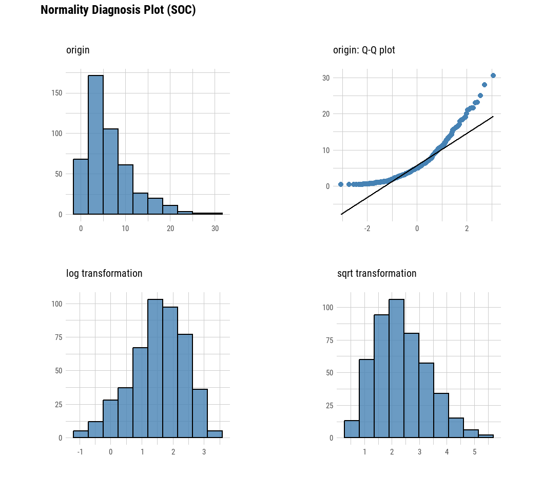

Descriptive Statistics

The describe() function from dloookr package computes descriptive statistics for numerical data. The descriptive statistics help determine the distribution of numerical variables.

The variables of the tbl_df object returned by describe() are as follows.

• n : number of observations excluding missing values

• na : number of missing values

• mean : arithmetic average

• sd : standard deviation

• se_mean : standard error mean. sd/sqrt(n)

• IQR : interquartile range (Q3-Q1)

• skewness : skewness

• kurtosis : kurtosis

• p25 : Q1. 25% percentile

• p50 : median. 50% percentile

• p75 : Q3. 75% percentile

• p01, p05, p10, p20, p30 : 1%, 5%, 20%, 30% percentiles

• p40, p60, p70, p80 : 40%, 60%, 70%, 80% percentiles

• p90, p95, p99, p100 : 90%, 95%, 99%, 100% percentiles

Code

# First select  numerical columns
des.stata<-mf %>% 
  dplyr::select(SOC, DEM, MAP, MAT, NDVI) %>%
 # then descrive them
  dlookr::describe()
flextable(des.stata)

described_variables	n	na	mean	sd	se_mean	IQR	skewness	kurtosis	p00	p01	p05	p10	p20	p25	p30	p40	p50	p60	p70	p75	p80	p90	p95	p99	p100
SOC	467	4	6.3507623	5.0454091	0.233473691	5.9440000	1.46472837	2.4271923	0.4080000	0.4909400	0.9637000	1.2902000	2.3294000	2.7695000	3.1114000	3.9906000	4.9710000	6.1266000	7.5030000	8.7135000	10.0522000	13.3830000	16.5219000	22.1247600	30.4730000
DEM	471	0	1,631.1063061	767.6923254	35.373395140	1,058.9335335	-0.02350235	-0.8039161	258.6488037	288.9806610	353.7696533	441.8609924	925.0328369	1,175.3313595	1,271.5794680	1,400.3239750	1,592.8931880	1,876.8692630	2,164.8010250	2,234.2648930	2,334.0241700	2,620.1455080	2,797.0867920	3,157.0538086	3,618.0241700
MAP	471	0	499.3729530	206.9359198	9.535103866	237.6524048	1.08253930	0.4698226	193.9132233	205.0283020	261.5091248	290.6307068	340.8447266	352.7745056	371.9525452	404.3808899	432.6304016	471.3896484	557.4978027	590.4269104	663.0267944	835.6693726	927.7701416	1,102.3618041	1,128.1145020
MAT	471	0	8.8855211	4.0981336	0.188832030	6.5642326	-0.27522458	-0.8236567	-0.5910638	-0.1158469	1.6258606	2.9455154	5.0193229	5.8800533	6.8264499	7.5748353	9.1728353	10.5665998	11.8026342	12.4442859	12.7931766	13.9399471	14.6389923	16.2291578	16.8742866
NDVI	471	0	0.4354311	0.1620239	0.007465669	0.2505557	0.23375088	-0.9180418	0.1424335	0.1631678	0.1920738	0.2215059	0.2756113	0.3053468	0.3317074	0.3769788	0.4156825	0.4773465	0.5348566	0.5559025	0.5853671	0.6759516	0.7216224	0.7601239	0.7969922

The describe() function supports the group_by() function syntax of the dplyr package. Following function calculate descriptive testatrices of SOC and NDVI of different NLCD

Code

mf %>%
  group_by(NLCD) %>% 
  dlookr::describe(SOC, NDVI) %>%
  flextable()

described_variables	NLCD	n	na	mean	sd	se_mean	IQR	skewness	kurtosis	p00	p01	p05	p10	p20	p25	p30	p40	p50	p60	p70	p75	p80	p90	p95	p99	p100
NDVI	Forest	93	0	0.5705648	0.1155016	0.01197696	0.1165678	-0.6719584	0.1157272	0.2830779	0.2856635	0.3427034	0.3610759	0.5045352	0.5326702	0.5390721	0.5576768	0.5759758	0.6085463	0.6290170	0.6492380	0.6708930	0.7010803	0.7353695	0.7711932	0.7814745
NDVI	Herbaceous	151	0	0.4003131	0.1307054	0.01063666	0.1257634	0.9764992	0.4084170	0.1648289	0.1785699	0.2555612	0.2651424	0.2944161	0.3124843	0.3308861	0.3497368	0.3769788	0.3934043	0.4193905	0.4382476	0.4771240	0.6033114	0.6916735	0.7305025	0.7337248
NDVI	Planted/Cultivated	97	0	0.5332255	0.1213052	0.01231668	0.1373269	0.5177150	-0.6469923	0.3249635	0.3262391	0.3740784	0.3937608	0.4236221	0.4498498	0.4584951	0.4879352	0.5132312	0.5297822	0.5670107	0.5871767	0.6677204	0.7226615	0.7493749	0.7969922	0.7969922
NDVI	Shrubland	130	0	0.3065798	0.1295559	0.01136280	0.1688918	1.1160872	0.4843057	0.1424335	0.1501656	0.1663934	0.1871671	0.2014691	0.2101985	0.2158819	0.2352937	0.2691359	0.2868186	0.3441049	0.3790904	0.4145865	0.5239458	0.5461648	0.6790463	0.6939532
SOC	Forest	93	0	10.4308817	6.8021471	0.70534979	10.3720000	0.7778065	-0.1552659	1.3330000	1.3578400	2.3656000	3.3538000	4.4686000	4.9310000	5.1440000	6.5884000	8.9740000	11.1936000	13.7130000	15.3030000	16.6020000	20.8730000	22.2096000	28.1831200	30.4730000
SOC	Herbaceous	150	1	5.4769667	3.9250913	0.32048236	4.3425000	1.2775572	1.4077233	0.4080000	0.5794500	1.0895000	1.4265000	2.2820000	2.6240000	3.0726000	3.5692000	4.6090000	5.2000000	6.3490000	6.9665000	8.2500000	11.0768000	13.3133500	17.5073200	18.8140000
SOC	Planted/Cultivated	97	0	6.6967216	3.5983014	0.36535215	5.4170000	0.5350421	-0.2587066	0.4620000	0.7192800	1.6380000	2.4642000	3.6094000	4.0020000	4.3260000	5.3820000	6.2300000	7.2166000	8.0810000	9.4190000	10.1170000	11.3962000	13.1846000	15.7638400	16.3360000
SOC	Shrubland	127	3	4.1307638	3.7448591	0.33230251	4.3105000	1.7061821	2.9893653	0.4460000	0.4746400	0.6162000	0.8046000	1.1344000	1.3500000	1.6174000	2.4386000	2.9960000	3.7474000	4.9050000	5.6605000	6.2840000	9.0786000	12.2261000	15.8518000	19.0990000

Correlation Analysis

correlate() calculates the correlation coefficient of all combinations of several numerical variables as follows:

Code

# First select  numerical columns
mf %>% 
  dplyr::select(SOC, DEM, MAP, MAT, NDVI) %>%
# then diagnose them
  dlookr::correlate()%>% 
  flextable()

var1	var2	coef_corr
DEM	SOC	0.16668949
MAP	SOC	0.49886194
MAT	SOC	-0.35802586
NDVI	SOC	0.58704521
SOC	DEM	0.16668949
MAP	DEM	-0.30672789
MAT	DEM	-0.80753239
NDVI	DEM	-0.06733319
SOC	MAP	0.49886194
DEM	MAP	-0.30672789
MAT	MAP	0.06032649
NDVI	MAP	0.80528269
SOC	MAT	-0.35802586
DEM	MAT	-0.80753239
MAP	MAT	0.06032649
NDVI	MAT	-0.20967449
SOC	NDVI	0.58704521
DEM	NDVI	-0.06733319
MAP	NDVI	0.80528269
MAT	NDVI	-0.20967449

The correlate() also supports the group_by() function syntax in the dplyr package.

Code

mf %>% 
  group_by(NLCD) %>%
  dplyr::select(SOC, DEM, MAP, MAT, NDVI) %>%
# then diagnose them
  dlookr::correlate()%>% 
  flextable()

NLCD	var1	var2	coef_corr
Forest	DEM	SOC	0.30298598
Forest	MAP	SOC	0.48134776
Forest	MAT	SOC	-0.46258320
Forest	NDVI	SOC	0.39140504
Forest	SOC	DEM	0.30298598
Forest	MAP	DEM	0.41052474
Forest	MAT	DEM	-0.71735792
Forest	NDVI	DEM	0.39660074
Forest	SOC	MAP	0.48134776
Forest	DEM	MAP	0.41052474
Forest	MAT	MAP	-0.62794270
Forest	NDVI	MAP	0.63598331
Forest	SOC	MAT	-0.46258320
Forest	DEM	MAT	-0.71735792
Forest	MAP	MAT	-0.62794270
Forest	NDVI	MAT	-0.48149700
Forest	SOC	NDVI	0.39140504
Forest	DEM	NDVI	0.39660074
Forest	MAP	NDVI	0.63598331
Forest	MAT	NDVI	-0.48149700
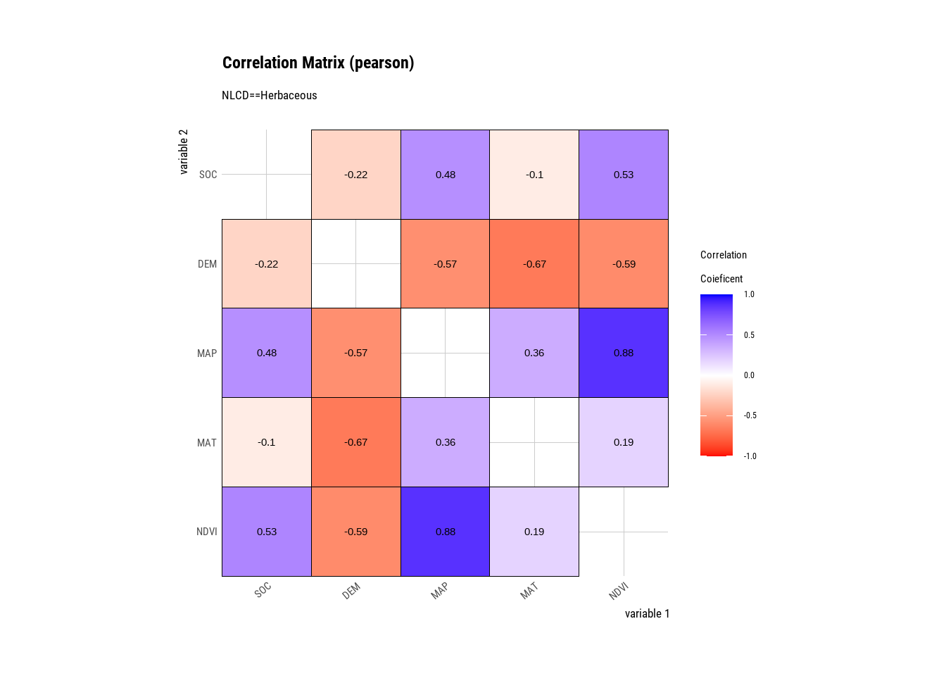
Herbaceous	DEM	SOC	-0.22121181
Herbaceous	MAP	SOC	0.48276882
Herbaceous	MAT	SOC	-0.10104174
Herbaceous	NDVI	SOC	0.52751680
Herbaceous	SOC	DEM	-0.22121181
Herbaceous	MAP	DEM	-0.57025818
Herbaceous	MAT	DEM	-0.66962468
Herbaceous	NDVI	DEM	-0.59258641
Herbaceous	SOC	MAP	0.48276882
Herbaceous	DEM	MAP	-0.57025818
Herbaceous	MAT	MAP	0.35544711
Herbaceous	NDVI	MAP	0.87783385
Herbaceous	SOC	MAT	-0.10104174
Herbaceous	DEM	MAT	-0.66962468
Herbaceous	MAP	MAT	0.35544711
Herbaceous	NDVI	MAT	0.18936050
Herbaceous	SOC	NDVI	0.52751680
Herbaceous	DEM	NDVI	-0.59258641
Herbaceous	MAP	NDVI	0.87783385
Herbaceous	MAT	NDVI	0.18936050
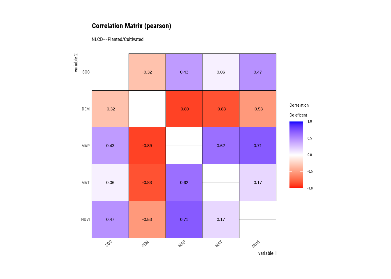
Planted/Cultivated	DEM	SOC	-0.31880666
Planted/Cultivated	MAP	SOC	0.42971838
Planted/Cultivated	MAT	SOC	0.06276231
Planted/Cultivated	NDVI	SOC	0.47472055
Planted/Cultivated	SOC	DEM	-0.31880666
Planted/Cultivated	MAP	DEM	-0.88745536
Planted/Cultivated	MAT	DEM	-0.83305530
Planted/Cultivated	NDVI	DEM	-0.52616146
Planted/Cultivated	SOC	MAP	0.42971838
Planted/Cultivated	DEM	MAP	-0.88745536
Planted/Cultivated	MAT	MAP	0.62195665
Planted/Cultivated	NDVI	MAP	0.71441683
Planted/Cultivated	SOC	MAT	0.06276231
Planted/Cultivated	DEM	MAT	-0.83305530
Planted/Cultivated	MAP	MAT	0.62195665
Planted/Cultivated	NDVI	MAT	0.17053661
Planted/Cultivated	SOC	NDVI	0.47472055
Planted/Cultivated	DEM	NDVI	-0.52616146
Planted/Cultivated	MAP	NDVI	0.71441683
Planted/Cultivated	MAT	NDVI	0.17053661
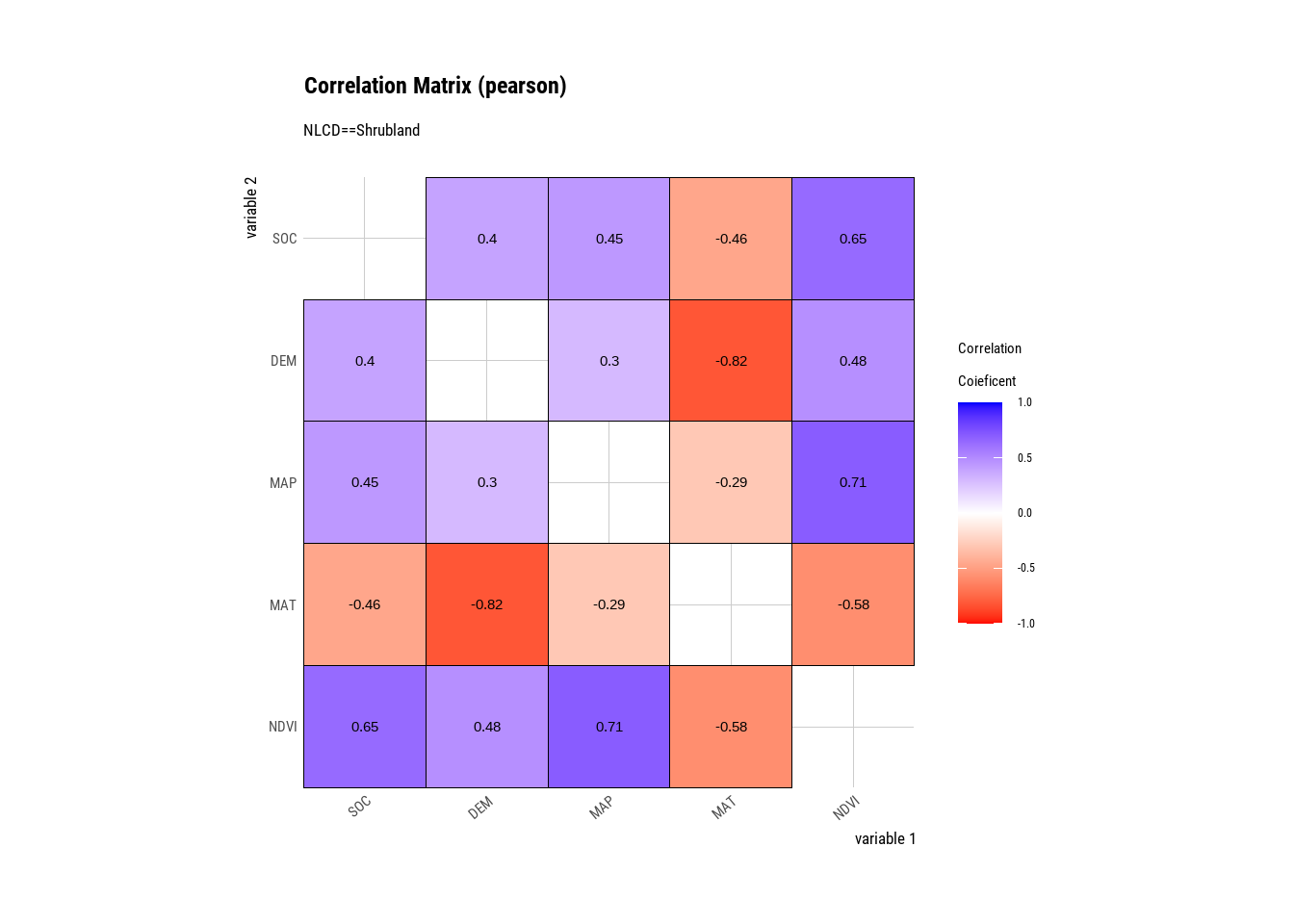
Shrubland	DEM	SOC	0.39720120
Shrubland	MAP	SOC	0.44532165
Shrubland	MAT	SOC	-0.45936785
Shrubland	NDVI	SOC	0.64602818
Shrubland	SOC	DEM	0.39720120
Shrubland	MAP	DEM	0.29834522
Shrubland	MAT	DEM	-0.81913433
Shrubland	NDVI	DEM	0.48180780
Shrubland	SOC	MAP	0.44532165
Shrubland	DEM	MAP	0.29834522
Shrubland	MAT	MAP	-0.28844730
Shrubland	NDVI	MAP	0.70639285
Shrubland	SOC	MAT	-0.45936785
Shrubland	DEM	MAT	-0.81913433
Shrubland	MAP	MAT	-0.28844730
Shrubland	NDVI	MAT	-0.57829256
Shrubland	SOC	NDVI	0.64602818
Shrubland	DEM	NDVI	0.48180780
Shrubland	MAP	NDVI	0.70639285
Shrubland	MAT	NDVI	-0.57829256

Visualization of the Correlation Matrix

plot.correlate() visualizes the correlation matrix.

Code

mf %>% 
  dplyr::select(SOC, DEM, MAP, MAT, NDVI) %>%
# then diagnose them
  dlookr::correlate()%>% 
  plot()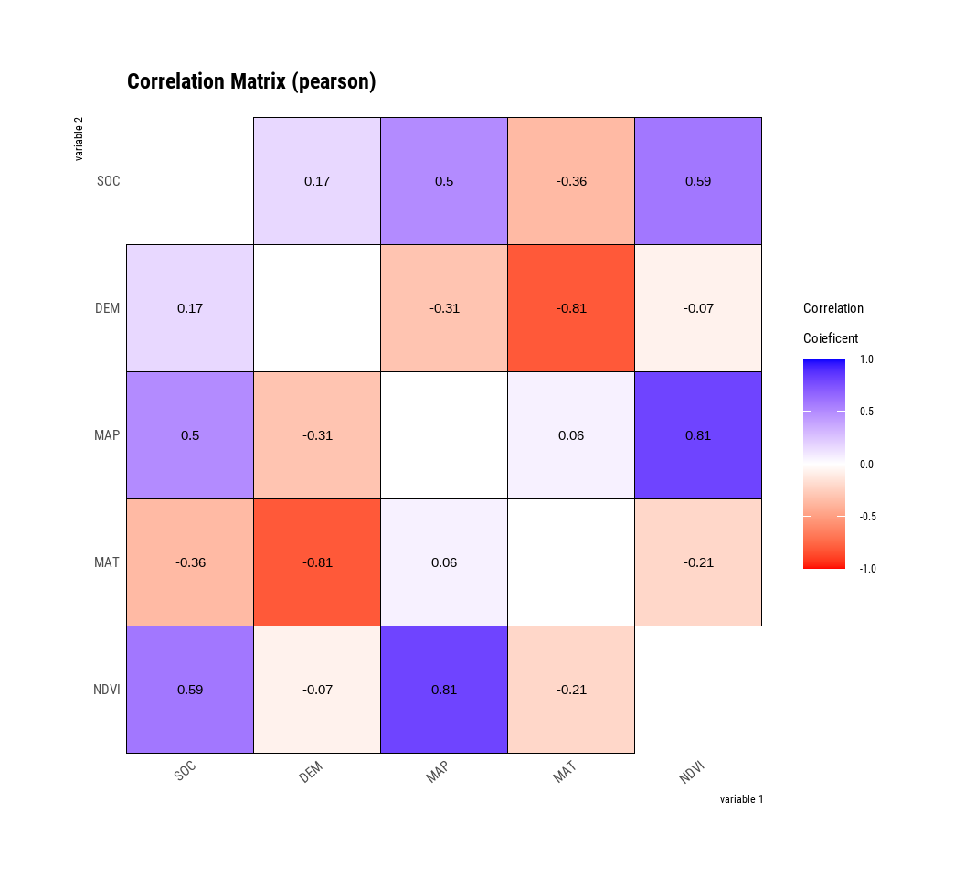

The plot.correlate() function also supports the group_by() function syntax in the dplyr package.

Code

mf %>% 
  group_by(NLCD) %>%
  dplyr::select(SOC, DEM, MAP, MAT, NDVI) %>%
# then diagnose them
  dlookr::correlate()%>% 
  plot()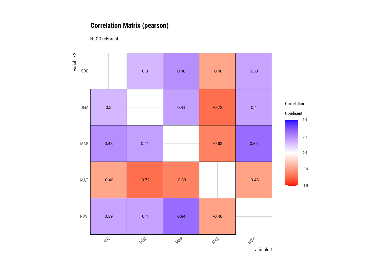

Exercise

1. Create a R-Markdown documents (name homework_04.rmd) in this project and do all Tasks ( using the data shown below.

2. Submit all codes and output as a HTML document (homework_04.html) before class of next week.

Required R-Package

tidyverse and dlookr.

Data

bd_arsenic_data_raw.csv

Download the data and save in your project directory. Use read_csv to load the data in your R-session. For example:

mf<-read_csv(“bd_arsenic_data_raw.csv”))

Tasks

1. Use dlookr::diagnose() function of dlookr package to do Data Quality Diagnosis all variables

2. Use dlookr::diagnose_numeric(), diagnoses numeric such as GAs,StAs, WAs, SAs, SPAs,SAoAs and SAoFe

3. Use dlookr::diagnose_category() to diagnoses the categorical variables (Land_type and variety) of a data frame.

4. Use dlookr::diagnose_outlier() to diagnosis outlier of GAs, StAs, WAs, and SAs.

5. Use dlookr::plot_outlier() to visualizes outliers of SAs

6. Performs a normality test on multiple numerical data (such as GAs,StAs, WAs,SAs, SPAs,SAoAs and SAoFe) using dlookr::normality() function, .

7. Use dlookr::normality() and dplyr::group_by() check normality of rice garin As (GAs) in different rice varieties.

8. Plot histogram and QQ-plot of SAs and histogram and square root transformed SAs using dlookr::plot_normality() function

9. Create a descriptive statistics table for GAs, StAs, Soil, WAs, PAs using dlookr::describe() and flextable() functions

10. Use dlookr::describe() and dplyr::group_by() functions calculate descriptive testatrices of SAs, SPAs, SAoAs and SAoFe in different landtypes

11. Calculates the correlation coefficient of all combinations of WAs, WFe, WP, WEc, SEc, SAs, SPAs, SAoAs and SAoFe and plot them using dlookr::correlate() and plot() functions.

12. Calculates the correlation coefficients in two landtypes: use dlookr::correlate() and dplyr::group_by()

Further Reading

1. dlook

2. Package dlookr

3. R package reviews-dlookr