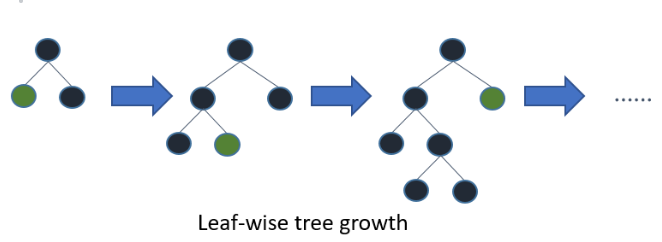
Light Gradient Boosting Machine (LightGBM)

LightGBM (Light Gradient Boosting Machine) is an open-source gradient boosting framework that is designed to be both efficient and scalable. It is based on the gradient boosting framework and uses a tree-based learning algorithm. LightGBM uses a novel technique called “Gradient-based One-Side Sampling” (GOSS) to achieve a faster and more accurate training process. It also uses a “Leaf-wise” strategy, which grows the tree by splitting the leaf that yields the maximum reduction in the loss function, resulting in a more balanced and less deep tree.

Note

Gradient-based One-Side Sampling” (GOSS):

Gradient-based One-Side Sampling (GOSS) is a data subsampling method used in LightGBM. GOSS is designed to speed up the training process of gradient boosting algorithms while maintaining or improving the model’s accuracy.GOSS works by first sorting the training instances according to their gradients. The instances with larger gradients are considered more important for the model, as they provide more information about the loss function

The key benefits of LightGBM are its speed, scalability, and accuracy. It can handle large-scale datasets with millions of samples and thousands of features, making it ideal for big data scenarios. It also has a smaller memory footprint compared to other gradient boosting algorithms, which makes it easier to train models on limited memory resources. It is designed to be distributed and efficient with the following advantages:

Faster training speed and higher efficiency.
Lower memory usage.
Better accuracy.
Support of parallel, distributed, and GPU learning.
Capable of handling large-scale data.

GBM (Gradient Boosting Machine) and LightGBM (Light Gradient Boosting Machine) are both gradient boosting algorithms used for supervised learning problems. While they share the same general approach to model training, there are several key differences between the two algorithms:

Speed: LightGBM is generally faster than GBM. This is because it uses a more efficient algorithm for finding the best split points, and it employs parallel processing to speed up the training process.
Memory Usage: LightGBM has a smaller memory footprint than GBM, which allows it to handle larger datasets with high-dimensional features.
Categorical Features Handling: LightGBM has built-in support for handling categorical features, which can be a common feature type in real-world datasets. GBM does not have this feature.
Leaf-wise Growth: LightGBM uses a “Leaf-wise” growth strategy, which grows the tree by splitting the leaf that yields the maximum reduction in the loss function, resulting in a more balanced and less deep tree. GBM uses a “Level-wise” growth strategy, which grows the tree level-by-level, resulting in a deeper and more unbalanced tree.

Note

Leaf-wise Growth:

“Leaf-wise” growth strategy is a tree building algorithm used in gradient boosting algorithms such as LightGBM. In this strategy, the tree is grown leaf-wise, meaning that it starts by growing the tree with a single root node, and then at each step, it selects the leaf node that yields the largest reduction in the loss function, and splits it into two child nodes

Sampling Techniques: LightGBM uses various sampling techniques to speed up the training process, such as Gradient-based One-Side Sampling (GOSS) and Exclusive Feature Bundling (EFB), which can improve the efficiency of the algorithm without sacrificing accuracy.

In summary, LightGBM is a fast and efficient gradient boosting framework that can handle large datasets with high-dimensional features. Its unique GOSS technique and Leaf-wise strategy make it a powerful tool for building accurate and scalable machine learning models.

Light Gradient Boosting Machine (lightGBM) with “lightgbm” package

The LightGBM R package provides an implementation of the LightGBM algorithm, a highly efficient gradient boosting framework. Here are some key features of the LightGBM R package:

High performance: LightGBM is designed to be highly efficient and scalable, making it well-suited for large datasets and high-dimensional feature spaces. The R package provides an interface to the underlying C++ library, which allows it to take advantage of multi-threading and other optimization techniques.
Cross-validation: The LightGBM R package provides tools for cross-validation, which can be used to tune hyperparameters and assess model performance.
Feature importance: LightGBM computes the feature importance by measuring the number of times each feature is split on in the tree building process. The more a feature is used for splitting, the more important it is considered to be. The R package provides functions for visualizing the feature importance and selecting the most important features.
Regularization: LightGBM provides several regularization techniques, such as L1 and L2 regularization, to prevent overfitting. The R package provides options for controlling the amount of regularization.
Missing value handling: LightGBM can handle missing values in the data, using a default direction at each node to handle missing values.
Flexibility: LightGBM can be used for a wide range of machine learning tasks, including regression, classification, and ranking. It can also handle both numerical and categorical features, and supports custom objective functions.
GPU acceleration: The LightGBM R package supports GPU acceleration, which can significantly speed up training and inference on compatible hardware.

Install the LightGbm R package from CRAN using the following command:

install.packages(“lightgbm”)

Code

library(lightgbm)

Data

In this exercise we will use following data set and use DEM, MAP, MAT, NAVI, NLCD, NLCD, and FRG to fit LightGbm regression model.

gp_soil_data.csv

Code

library(tidyverse)
# define data folder
urlfile = "https://github.com//zia207/r-colab/raw/main/Data/USA/gp_soil_data.csv"
mf<-read_csv(url(urlfile))
# Create a data-frame
df<-mf %>% dplyr::select(SOC, DEM, Slope, Aspect, TPI, KFactor, SiltClay, MAT, MAP,NDVI, NLCD, FRG)%>%
    glimpse()

Rows: 467
Columns: 12
$ SOC      <dbl> 15.763, 15.883, 18.142, 10.745, 10.479, 16.987, 24.954, 6.288…
$ DEM      <dbl> 2229.079, 1889.400, 2423.048, 2484.283, 2396.195, 2360.573, 2…
$ Slope    <dbl> 5.6716146, 8.9138117, 4.7748051, 7.1218114, 7.9498644, 9.6632…
$ Aspect   <dbl> 159.1877, 156.8786, 168.6124, 198.3536, 201.3215, 208.9732, 2…
$ TPI      <dbl> -0.08572358, 4.55913162, 2.60588670, 5.14693117, 3.75570583, …
$ KFactor  <dbl> 0.31999999, 0.26121211, 0.21619999, 0.18166667, 0.12551020, 0…
$ SiltClay <dbl> 64.84270, 72.00455, 57.18700, 54.99166, 51.22857, 45.02000, 5…
$ MAT      <dbl> 4.5951686, 3.8599243, 0.8855000, 0.4707811, 0.7588266, 1.3586…
$ MAP      <dbl> 468.3245, 536.3522, 859.5509, 869.4724, 802.9743, 1121.2744, …
$ NDVI     <dbl> 0.4139390, 0.6939532, 0.5466033, 0.6191013, 0.5844722, 0.6028…
$ NLCD     <chr> "Shrubland", "Shrubland", "Forest", "Forest", "Forest", "Fore…
$ FRG      <chr> "Fire Regime Group IV", "Fire Regime Group IV", "Fire Regime …

Data Preparation

Code

library(fastDummies)
tmp <- df[, c(11:12)]
# create dummy variables
tmp1 <- dummy_cols(tmp)
tmp1 <- tmp1[,3:12]

# create a dataframe
d <- data.frame(df[, c(1:10)], tmp1)
m <- as.matrix(d)

Create training and test dataset

Code

library(caret)
set.seed(123)
indices <- sample(1:nrow(df), size = 0.75 * nrow(df))
train <- m[indices,]
test <- m[-indices,]

Load the train and test data into the LightGBM dataset object

Code

y_train <- train[,1]
y_test <- test[,1]
train_lgb <- lgb.Dataset(train[,2:20],label=y_train)
test_lgb <- lgb.Dataset.create.valid(train_lgb,test[,2:20],label = y_test)

Fit lightGBM model

Next, we’ll fit the XGBoost model by using the lgb.train() function, which displays the training and testing RMSE (root mean squared error) for each round of boosting

Code

lightgbm_model <- lgb.train(
  params = list(
    objective = "regression", 
    metric = "l2"
  ), 
  data = train_lgb
)

[LightGBM] [Warning] Auto-choosing col-wise multi-threading, the overhead of testing was 0.002636 seconds.
You can set `force_col_wise=true` to remove the overhead.
[LightGBM] [Info] Total Bins 1069
[LightGBM] [Info] Number of data points in the train set: 350, number of used features: 16
[LightGBM] [Info] Start training from score 6.263474
[LightGBM] [Warning] No further splits with positive gain, best gain: -inf
[LightGBM] [Warning] No further splits with positive gain, best gain: -inf
[LightGBM] [Warning] No further splits with positive gain, best gain: -inf
[LightGBM] [Warning] No further splits with positive gain, best gain: -inf
[LightGBM] [Warning] No further splits with positive gain, best gain: -inf
[LightGBM] [Warning] No further splits with positive gain, best gain: -inf
[LightGBM] [Warning] No further splits with positive gain, best gain: -inf
[LightGBM] [Warning] No further splits with positive gain, best gain: -inf
[LightGBM] [Warning] No further splits with positive gain, best gain: -inf
[LightGBM] [Warning] No further splits with positive gain, best gain: -inf
[LightGBM] [Warning] No further splits with positive gain, best gain: -inf
[LightGBM] [Warning] No further splits with positive gain, best gain: -inf
[LightGBM] [Warning] No further splits with positive gain, best gain: -inf
[LightGBM] [Warning] No further splits with positive gain, best gain: -inf
[LightGBM] [Warning] No further splits with positive gain, best gain: -inf
[LightGBM] [Warning] No further splits with positive gain, best gain: -inf
[LightGBM] [Warning] No further splits with positive gain, best gain: -inf
[LightGBM] [Warning] No further splits with positive gain, best gain: -inf
[LightGBM] [Warning] No further splits with positive gain, best gain: -inf
[LightGBM] [Warning] No further splits with positive gain, best gain: -inf
[LightGBM] [Warning] No further splits with positive gain, best gain: -inf
[LightGBM] [Warning] No further splits with positive gain, best gain: -inf
[LightGBM] [Warning] No further splits with positive gain, best gain: -inf
[LightGBM] [Warning] No further splits with positive gain, best gain: -inf
[LightGBM] [Warning] No further splits with positive gain, best gain: -inf
[LightGBM] [Warning] No further splits with positive gain, best gain: -inf
[LightGBM] [Warning] No further splits with positive gain, best gain: -inf
[LightGBM] [Warning] No further splits with positive gain, best gain: -inf
[LightGBM] [Warning] No further splits with positive gain, best gain: -inf
[LightGBM] [Warning] No further splits with positive gain, best gain: -inf
[LightGBM] [Warning] No further splits with positive gain, best gain: -inf
[LightGBM] [Warning] No further splits with positive gain, best gain: -inf
[LightGBM] [Warning] No further splits with positive gain, best gain: -inf
[LightGBM] [Warning] No further splits with positive gain, best gain: -inf
[LightGBM] [Warning] No further splits with positive gain, best gain: -inf
[LightGBM] [Warning] No further splits with positive gain, best gain: -inf
[LightGBM] [Warning] No further splits with positive gain, best gain: -inf
[LightGBM] [Warning] No further splits with positive gain, best gain: -inf
[LightGBM] [Warning] No further splits with positive gain, best gain: -inf
[LightGBM] [Warning] No further splits with positive gain, best gain: -inf
[LightGBM] [Warning] No further splits with positive gain, best gain: -inf
[LightGBM] [Warning] No further splits with positive gain, best gain: -inf
[LightGBM] [Warning] No further splits with positive gain, best gain: -inf
[LightGBM] [Warning] No further splits with positive gain, best gain: -inf
[LightGBM] [Warning] No further splits with positive gain, best gain: -inf
[LightGBM] [Warning] No further splits with positive gain, best gain: -inf
[LightGBM] [Warning] No further splits with positive gain, best gain: -inf
[LightGBM] [Warning] No further splits with positive gain, best gain: -inf
[LightGBM] [Warning] No further splits with positive gain, best gain: -inf
[LightGBM] [Warning] No further splits with positive gain, best gain: -inf
[LightGBM] [Warning] No further splits with positive gain, best gain: -inf
[LightGBM] [Warning] No further splits with positive gain, best gain: -inf
[LightGBM] [Warning] No further splits with positive gain, best gain: -inf
[LightGBM] [Warning] No further splits with positive gain, best gain: -inf
[LightGBM] [Warning] No further splits with positive gain, best gain: -inf
[LightGBM] [Warning] No further splits with positive gain, best gain: -inf
[LightGBM] [Warning] No further splits with positive gain, best gain: -inf
[LightGBM] [Warning] No further splits with positive gain, best gain: -inf
[LightGBM] [Warning] No further splits with positive gain, best gain: -inf
[LightGBM] [Warning] No further splits with positive gain, best gain: -inf
[LightGBM] [Warning] No further splits with positive gain, best gain: -inf
[LightGBM] [Warning] No further splits with positive gain, best gain: -inf
[LightGBM] [Warning] No further splits with positive gain, best gain: -inf
[LightGBM] [Warning] No further splits with positive gain, best gain: -inf
[LightGBM] [Warning] No further splits with positive gain, best gain: -inf
[LightGBM] [Warning] No further splits with positive gain, best gain: -inf
[LightGBM] [Warning] No further splits with positive gain, best gain: -inf
[LightGBM] [Warning] No further splits with positive gain, best gain: -inf
[LightGBM] [Warning] No further splits with positive gain, best gain: -inf
[LightGBM] [Warning] No further splits with positive gain, best gain: -inf
[LightGBM] [Warning] No further splits with positive gain, best gain: -inf
[LightGBM] [Warning] No further splits with positive gain, best gain: -inf
[LightGBM] [Warning] No further splits with positive gain, best gain: -inf
[LightGBM] [Warning] No further splits with positive gain, best gain: -inf
[LightGBM] [Warning] No further splits with positive gain, best gain: -inf
[LightGBM] [Warning] No further splits with positive gain, best gain: -inf
[LightGBM] [Warning] No further splits with positive gain, best gain: -inf
[LightGBM] [Warning] No further splits with positive gain, best gain: -inf
[LightGBM] [Warning] No further splits with positive gain, best gain: -inf
[LightGBM] [Warning] No further splits with positive gain, best gain: -inf
[LightGBM] [Warning] No further splits with positive gain, best gain: -inf
[LightGBM] [Warning] No further splits with positive gain, best gain: -inf
[LightGBM] [Warning] No further splits with positive gain, best gain: -inf
[LightGBM] [Warning] No further splits with positive gain, best gain: -inf
[LightGBM] [Warning] No further splits with positive gain, best gain: -inf
[LightGBM] [Warning] No further splits with positive gain, best gain: -inf
[LightGBM] [Warning] No further splits with positive gain, best gain: -inf
[LightGBM] [Warning] No further splits with positive gain, best gain: -inf
[LightGBM] [Warning] No further splits with positive gain, best gain: -inf
[LightGBM] [Warning] No further splits with positive gain, best gain: -inf
[LightGBM] [Warning] No further splits with positive gain, best gain: -inf
[LightGBM] [Warning] No further splits with positive gain, best gain: -inf
[LightGBM] [Warning] No further splits with positive gain, best gain: -inf
[LightGBM] [Warning] No further splits with positive gain, best gain: -inf
[LightGBM] [Warning] No further splits with positive gain, best gain: -inf
[LightGBM] [Warning] No further splits with positive gain, best gain: -inf
[LightGBM] [Warning] No further splits with positive gain, best gain: -inf
[LightGBM] [Warning] No further splits with positive gain, best gain: -inf
[LightGBM] [Warning] No further splits with positive gain, best gain: -inf
[LightGBM] [Warning] No further splits with positive gain, best gain: -inf

Prediction

Code

yhat_fit_train <- predict(lightgbm_model,train[,2:20])
yhat_predict_test <- predict(lightgbm_model,test[,2:20])

Code

rmse_train <- RMSE(y_train,yhat_fit_train)
rmse_test <- RMSE(y_test,yhat_predict_test)
rmse_train

[1] 1.667434

Code

rmse_test

[1] 4.216184

Code

rm(list = ls())

Tunning LightGBM with tidymodel

The tidymodels provides a comprehensive framework for building, tuning, and evaluating LightGBM model while following the principles of the tidyverse.

Data

Code

library(tidyverse)
# define data folder
urlfile = "https://github.com//zia207/r-colab/raw/main/Data/USA/gp_soil_data.csv"
mf<-read_csv(url(urlfile))

# Create a data-frame
df<-mf %>% dplyr::select(SOC, DEM, Slope, Aspect, TPI, KFactor, SiltClay, MAT, MAP,NDVI, NLCD, FRG)%>%
    glimpse()

Rows: 467
Columns: 12
$ SOC      <dbl> 15.763, 15.883, 18.142, 10.745, 10.479, 16.987, 24.954, 6.288…
$ DEM      <dbl> 2229.079, 1889.400, 2423.048, 2484.283, 2396.195, 2360.573, 2…
$ Slope    <dbl> 5.6716146, 8.9138117, 4.7748051, 7.1218114, 7.9498644, 9.6632…
$ Aspect   <dbl> 159.1877, 156.8786, 168.6124, 198.3536, 201.3215, 208.9732, 2…
$ TPI      <dbl> -0.08572358, 4.55913162, 2.60588670, 5.14693117, 3.75570583, …
$ KFactor  <dbl> 0.31999999, 0.26121211, 0.21619999, 0.18166667, 0.12551020, 0…
$ SiltClay <dbl> 64.84270, 72.00455, 57.18700, 54.99166, 51.22857, 45.02000, 5…
$ MAT      <dbl> 4.5951686, 3.8599243, 0.8855000, 0.4707811, 0.7588266, 1.3586…
$ MAP      <dbl> 468.3245, 536.3522, 859.5509, 869.4724, 802.9743, 1121.2744, …
$ NDVI     <dbl> 0.4139390, 0.6939532, 0.5466033, 0.6191013, 0.5844722, 0.6028…
$ NLCD     <chr> "Shrubland", "Shrubland", "Forest", "Forest", "Forest", "Fore…
$ FRG      <chr> "Fire Regime Group IV", "Fire Regime Group IV", "Fire Regime …

Split data

Code

library(tidymodels)

── Attaching packages ────────────────────────────────────── tidymodels 1.1.0 ──

✔ broom        1.0.5     ✔ rsample      1.1.1
✔ dials        1.2.0     ✔ tune         1.1.1
✔ infer        1.0.4     ✔ workflows    1.1.3
✔ modeldata    1.1.0     ✔ workflowsets 1.0.1
✔ parsnip      1.1.0     ✔ yardstick    1.2.0
✔ recipes      1.0.6

── Conflicts ───────────────────────────────────────── tidymodels_conflicts() ──
✖ scales::discard()        masks purrr::discard()
✖ dplyr::filter()          masks stats::filter()
✖ recipes::fixed()         masks stringr::fixed()
✖ dplyr::lag()             masks stats::lag()
✖ caret::lift()            masks purrr::lift()
✖ yardstick::precision()   masks caret::precision()
✖ yardstick::recall()      masks caret::recall()
✖ yardstick::sensitivity() masks caret::sensitivity()
✖ dplyr::slice()           masks lightgbm::slice()
✖ yardstick::spec()        masks readr::spec()
✖ yardstick::specificity() masks caret::specificity()
✖ recipes::step()          masks stats::step()
• Use suppressPackageStartupMessages() to eliminate package startup messages

Code

set.seed(1245)   # for reproducibility
split <- initial_split(df, prop = 0.8, strata = SOC)
train <- split %>% training()
test <-  split %>% testing()

# Set 10 fold cross-validation data set 
cv_folds <- vfold_cv(train, v = 5)

Create Recipe

A recipe is a description of the steps to be applied to a data set in order to prepare it for data analysis. Before training the model, we can use a recipe to do some pre-processing required by the model.

Code

# Create a recipe
lightGBM_recipe <-
  recipe(SOC ~ ., data = train) %>%
  step_zv(all_predictors()) %>%
  step_dummy(all_nominal()) %>%
  step_normalize(all_numeric_predictors())

Specify tunable Hypermeters of LightGBM

Parsnip could not support an implementation for boost_tree regression model specifications using the lightgbm engine. The parsnip extension package “bonsai” implements support for this specification. We need to install it and load to continue.

install.packages(“bonsai”)

According to the lightgbm parameter tuning guide the hyperparameters number of leaves, min_data_in_leaf, and max_depth are the most important features. Currently implemented for lightgbm in (treesnip) are:

feature_fraction (mtry)
num_iterations (trees)
min_data_in_leaf (min_n)
max_depth (tree_depth)
learning_rate (learn_rate)
min_gain_to_split (loss_reduction)
bagging_fraction (sample_size)

Code

library(bonsai)

lightgbm_model<-
  boost_tree(
    mtry = 5, 
    trees = 100, 
    min_n = tune(), 
    tree_depth = tune(),
    loss_reduction = tune(), 
    learn_rate = tune(), 
    sample_size = 0.75
  ) %>% 
  set_mode("regression") %>%
  set_engine("lightgbm")

lightgbm_model

Boosted Tree Model Specification (regression)

Main Arguments:
  mtry = 5
  trees = 100
  min_n = tune()
  tree_depth = tune()
  learn_rate = tune()
  loss_reduction = tune()
  sample_size = 0.75

Computational engine: lightgbm

Create Workflow

Code

lightgbm_wf <- workflow() %>% 
    add_model(lightgbm_model) %>% 
    add_recipe(lightGBM_recipe)

lightgbm_wf

══ Workflow ════════════════════════════════════════════════════════════════════
Preprocessor: Recipe
Model: boost_tree()

── Preprocessor ────────────────────────────────────────────────────────────────
3 Recipe Steps

• step_zv()
• step_dummy()
• step_normalize()

── Model ───────────────────────────────────────────────────────────────────────
Boosted Tree Model Specification (regression)

Main Arguments:
  mtry = 5
  trees = 100
  min_n = tune()
  tree_depth = tune()
  learn_rate = tune()
  loss_reduction = tune()
  sample_size = 0.75

Computational engine: lightgbm

Define random grid prameters

Code

lightgbm_grid <- parameters(lightgbm_model) %>% 
    finalize(train) %>% 
    grid_random(size = 20)
head(lightgbm_grid)

# A tibble: 6 × 4
  min_n tree_depth    learn_rate loss_reduction
  <int>      <int>         <dbl>          <dbl>
1     5          4 0.0498               1.71e-8
2     2         11 0.0000276            2.75e-7
3    39          9 0.000000453          3.09e-9
4    17         12 0.00000000325        1.71e-8
5    13          1 0.00000277           1.23e-8
6    28          9 0.0623               1.29e+1

Tune Grid

Code

doParallel::registerDoParallel()

set.seed(345)
# grid search
lightgbm_tune_grid <- lightgbm_wf %>%
    tune_grid(
        resamples = cv_folds,
        grid = lightgbm_grid,
        control = control_grid(verbose = F),
        metrics = metric_set(rmse, rsq, mae)
    )

Code

collect_metrics(lightgbm_tune_grid )

# A tibble: 60 × 10
   min_n tree_depth    learn_rate loss_reduction .metric .estimator  mean     n
   <int>      <int>         <dbl>          <dbl> <chr>   <chr>      <dbl> <int>
 1     5          4 0.0498         0.0000000171  mae     standard   2.85      5
 2     5          4 0.0498         0.0000000171  rmse    standard   4.01      5
 3     5          4 0.0498         0.0000000171  rsq     standard   0.375     5
 4     2         11 0.0000276      0.000000275   mae     standard   3.80      5
 5     2         11 0.0000276      0.000000275   rmse    standard   5.00      5
 6     2         11 0.0000276      0.000000275   rsq     standard   0.380     5
 7    39          9 0.000000453    0.00000000309 mae     standard   3.80      5
 8    39          9 0.000000453    0.00000000309 rmse    standard   5.00      5
 9    39          9 0.000000453    0.00000000309 rsq     standard   0.364     5
10    17         12 0.00000000325  0.0000000171  mae     standard   3.80      5
# ℹ 50 more rows
# ℹ 2 more variables: std_err <dbl>, .config <chr>

Code

autoplot(lightgbm_tune_grid)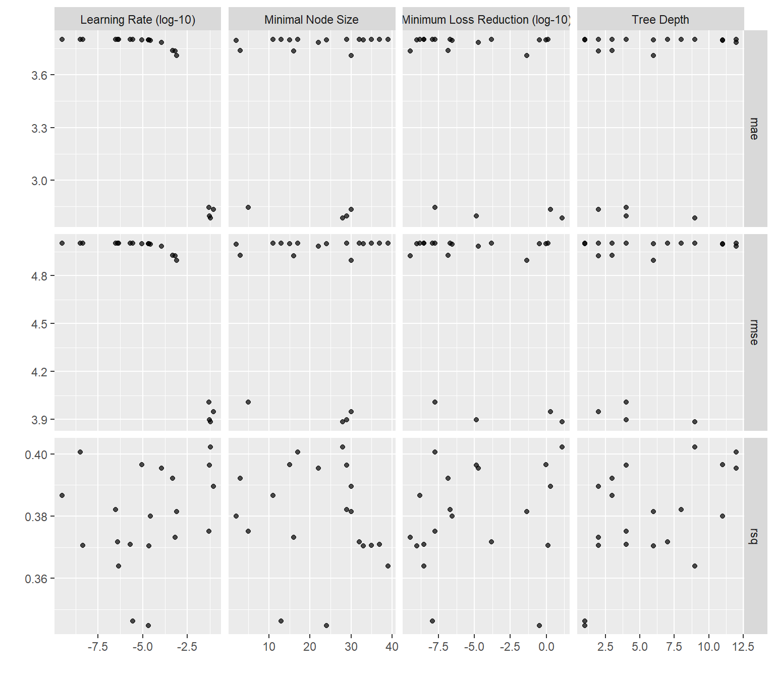

The best lightgbm model

Code

best_rmse <- select_best(lightgbm_tune_grid , "rmse")

lightgbm_final <- finalize_model(
  lightgbm_model,
  best_rmse
)

lightgbm_final

Boosted Tree Model Specification (regression)

Main Arguments:
  mtry = 5
  trees = 100
  min_n = 28
  tree_depth = 9
  learn_rate = 0.0623082219881162
  loss_reduction = 12.8917083526204
  sample_size = 0.75

Computational engine: lightgbm

Fit the model

We can either fit final_tree to training data using fit() or to the testing/training split using last_fit(), which will give us some other results along with the fitted output.

Code

final_fit <- fit(lightgbm_final, SOC ~ .,train)

Prediction

Code

test$SOC.pred = predict(final_fit,test)

Code

library(Matrix)
RMSE<- Metrics::rmse(test$SOC, test$SOC.pred$.pred)
RMSE

[1] 3.379888

Code

library(ggpmisc)
formula<-y~x

ggplot(test, aes(SOC,SOC.pred$.pred)) +
  geom_point() +
  geom_smooth(method = "lm")+
  stat_poly_eq(use_label(c("eq", "adj.R2")), formula = formula) +
  ggtitle("LightGBM") +
  xlab("Observed") + ylab("Predicted") +
  scale_x_continuous(limits=c(0,25), breaks=seq(0, 25, 5))+ 
  scale_y_continuous(limits=c(0,25), breaks=seq(0, 25, 5)) +
  # Flip the bars
  theme(
    panel.background = element_rect(fill = "grey95",colour = "gray75",size = 0.5, linetype = "solid"),
    axis.line = element_line(colour = "grey"),
    plot.title = element_text(size = 14, hjust = 0.5),
    axis.title.x = element_text(size = 14),
    axis.title.y = element_text(size = 14),
    axis.text.x=element_text(size=13, colour="black"),
    axis.text.y=element_text(size=13,angle = 90,vjust = 0.5, hjust=0.5, colour='black'))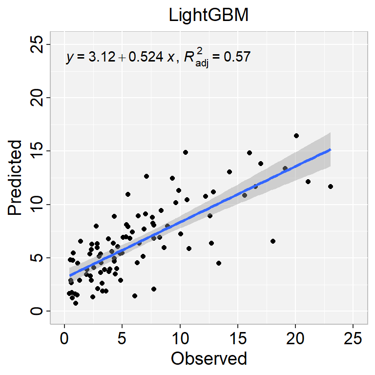

Variable Importance

Code

extract_fit_engine(final_fit) %>% 
  lightgbm::lgb.importance() %>% 
  lightgbm::lgb.plot.importance(top_n = 10)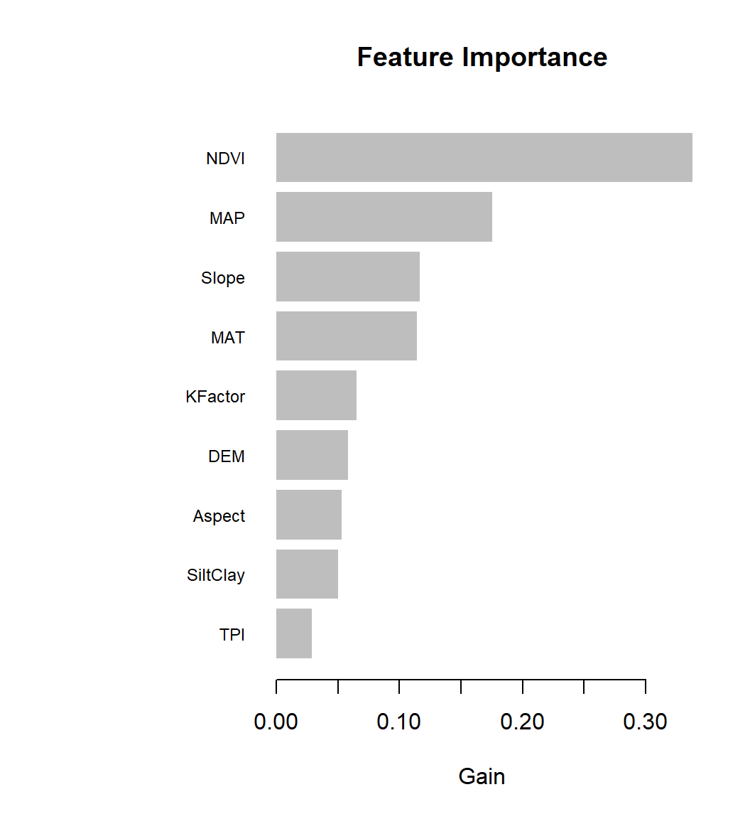

Exercise

Create a R-Markdown documents (name homework_15.rmd) in this project and do all Tasks using the data shown below.
Submit all codes and output as a HTML document (homework_15.html) before class of next week.

Required R-Package

tidyverse, caret, Metrics, tidymodels, vip, bonsai

Data

bd_soil_update.csv

Download the data and save in your project directory. Use read_csv to load the data in your R-session. For example:

mf<-read_csv(“bd_soil_update.csv”)

Tasks

Create a data-frame with following variables for Rajshahi Division:

First use filter() to select data from Rajshai division and then use select() functions to create data-frame with following variables:

SOM, DEM, NDVI, NDFI,

Tune, Fit and show the model performance of a lightgbm model with using tidymodel package

YouTube Video

What is Light GBM and how does it compare against XGBoost?

Source: DigitalSreeni

Light Gradient Boosting Machine (LightGBM)

Light Gradient Boosting Machine (lightGBM) with “lightgbm” package

Data

Data Preparation

Create training and test dataset

Load the train and test data into the LightGBM dataset object

Fit lightGBM model

Prediction

Tunning LightGBM with tidymodel

Data

Split data

Create Recipe

Specify tunable Hypermeters of LightGBM

Create Workflow

Define random grid prameters

Tune Grid

The best lightgbm model

Fit the model

Prediction

Variable Importance

Exercise

Required R-Package

Data

Tasks

Further Reading

YouTube Video