Random Forest (RF) is a tree-based machine learning algorithm that is used for classification, regression and other tasks in data analysis. It is a popular and robust algorithm that builds multiple decision trees and combines their predictions to make a final prediction. RF is a modification of Bagging (bootstrap aggregating) regression trees that builds a large collection of de-correlated trees and has become a very popular “out-of-the-box” learning algorithm that has low variance and higher predictive power than traditional bagging models.
Each decision tree in the Random Forest is constructed by randomly selecting a subset of the available features and then building a tree based on those features. This process is repeated a specified number of times, resulting in multiple decision trees. When a new data point needs to be classified, each tree in the forest is used to make a prediction, and the final prediction is based on the most common prediction made by all the trees.
Random Forest is a robust algorithm because it can handle large datasets with many features and is also resistant to overfitting, which can occur when a model is too complex and fits the training data too closely. Random Forest works by using ensemble learning, which means combining the predictions of multiple models to improve accuracy and reduce errors.
Here is how Random Forest works step by step:
Randomly select a subset of the dataset.
Construct a decision tree on the selected subset of the dataset.
Repeat steps 1 and 2 to construct multiple decision trees.
Pass each input through all the decision trees and record their outputs.
Determine the final output based on the majority vote (classification) or mean prediction (regression) of the decision trees.
Data
In this exercise we will use the following data set and use DEM, MAP, MAT, NAVI, NLCD, and FRG to fit an RF regression model.
The randomForest R package widely implements the random forest algorithm for building decision trees in machine learning. Random forests are an ensemble learning method that builds multiple decision trees and aggregates their predictions to make a final prediction. This can help to reduce overfitting and increase the accuracy of the model.
The randomForest package in R provides a simple interface for building random forests. It allows the user to specify the number of trees to build, the number of variables to sample at each split, and other hyperparameters. The package also includes functions for visualizing the random forest model, as well as methods for predicting new data and assessing model performance.
To get started with the randomForest package, you can install it from CRAN using the following code:
install.packages(“randomForest)
Code
library(randomForest)
Split Data
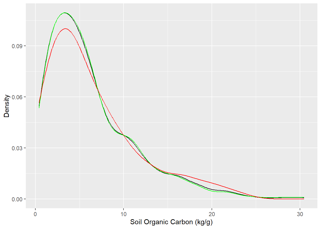
We use rsample package, install with tidymodels, to split data into training (70%) and test data (30%) set with Stratified Random Sampling. initial_split() creates a single binary split of the data into a training set and testing set.
Note
Stratified random sampling is a technique for selecting a representative sample from a population, where the sample is chosen in a way that ensures that certain subgroups within the population are adequately represented in the sample.
Code
##| fig.width: 4#| fig.height: 4library(tidymodels)set.seed(1245) # for reproducibilitysplit <-initial_split(df, prop =0.8, strata = SOC)train <- split %>%training()test <- split %>%testing()# Density plot all, train and test data ggplot()+geom_density(data = df, aes(SOC))+geom_density(data = train, aes(SOC), color ="green")+geom_density(data = test, aes(SOC), color ="red") +xlab("Soil Organic Carbon (kg/g)") +ylab("Density")
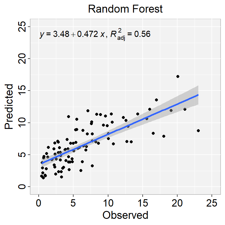
We can fit a random forest model using the randomForest() function, which implements Breiman’s random forest algorithm (based on Breiman and Cutler’s original Fortran code) for classification and regression. It can also be used in unsupervised mode for assessing proximities among data points.
Code
set.seed(123) # for reproducibilityrf.fit <-randomForest(SOC ~ ., data=train, ntree=100, # Number of trees to growmtry =8, # Number of variables randomly sampled as candidates at each split#sampsize = 0.65 , # Size(s) of sample to draw#nodesize = 5, # Minimum size of terminal nodes#maxnode = 5, # maximum number of terminal nodeskeep.forest =TRUE, importance=TRUE)
Code
rf.fit
Call:
 randomForest(formula = SOC ~ ., data = train, ntree = 100, mtry = 8,      keep.forest = TRUE, importance = TRUE)
               Type of random forest: regression
                     Number of trees: 100
No. of variables tried at each split: 8

          Mean of squared residuals: 16.6138
                    % Var explained: 33.72
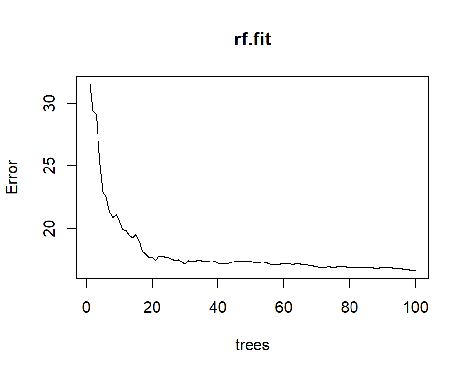
Plot RF model
Code
# Plotting modelplot(rf.fit)
Feature Importance
Feature importance in Random Forest refers to a measure of the contribution of each feature to the accuracy of the model. The importance of each feature is determined by calculating the relative influence of each variable: whether that variable was selected to split on during the tree building process, and how much the squared error (over all trees) improved (decreased) as a result. The importance of a feature is the sum of the importance of that feature across all decision trees in the Random Forest.
There are different methods to calculate feature importance in Random Forest. The most commonly used methods are:
Gini Importance: It measures the total reduction of the Gini index, which is a measure of impurity, that is achieved by each feature. A higher reduction in the Gini index indicates a higher importance of the feature.
Permutation Importance: It measures the decrease in the accuracy of the model when a feature is randomly permuted. A higher decrease in accuracy indicates a higher importance of the feature.
Mean Decrease Impurity:
In a Random Forest algorithm, node purity is a measure of how homogeneous the group of data points at a particular node is with respect to their target labels. The algorithm builds a decision tree by recursively splitting the data into smaller subsets based on the features and their values, with the aim of maximizing the node purity at each level.It measures the average reduction in impurity over all decision trees in the Random Forest when a feature is used to split a node. A higher reduction in impurity indicates a higher importance of the feature.
In regression, the feature importance is calculated based on the mean decrease in impurity of the regression tree nodes or measures the variability of the target variable within the node.. The impurity measure used for regression is the mean squared error (MSE) instead of the Gini index used in classification.
The importance of a feature is calculated by taking the total reduction in the MSE across all trees in the forest when the feature is used for splitting the nodes. A feature that reduces the MSE by a large amount is considered more important than a feature that reduces it by a smaller amount.
The feature importance scores can be normalized so that they add up to one. This allows for easy comparison of the relative importance of different features.
Once the feature importance is calculated, it can be used to select the most important features for the model or to interpret the model by understanding which features are driving the predictions.
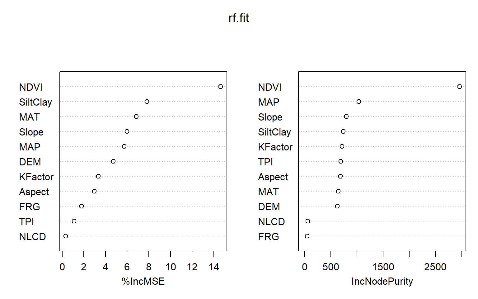
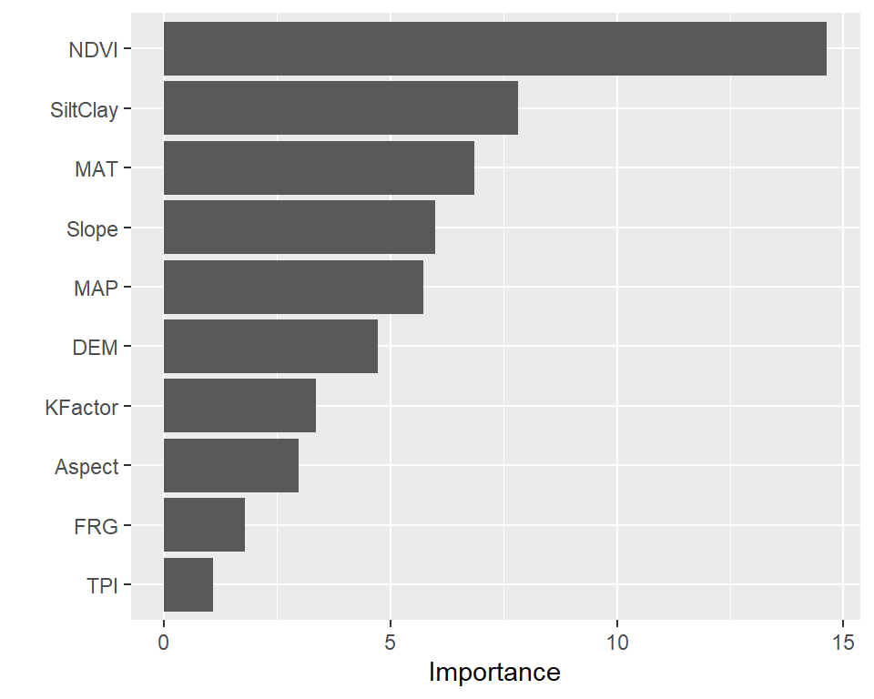
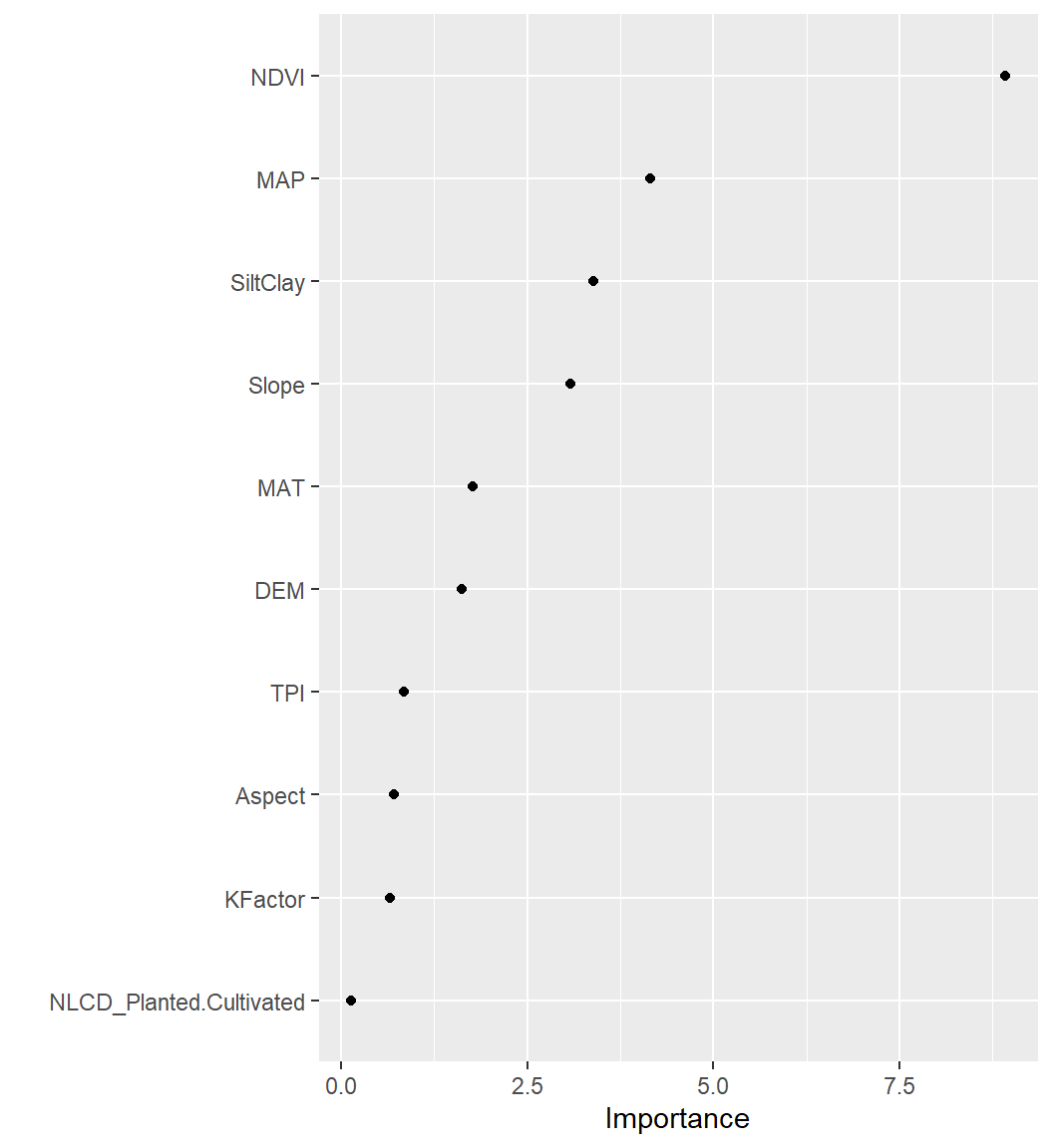
varImpPlot() function create dotchart of variable importance as measured by a Random Forest
Code
# Variable importance plotvarImpPlot(rf.fit)
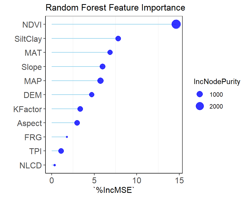
We can create a customize variable importance plot with ggplot2:
Code
# Get variable importance from the model fitImpData <-as.data.frame(importance(rf.fit))ImpData$Var.Names <-row.names(ImpData)# Plot importanceggplot(ImpData, aes(y=`%IncMSE`, x=reorder(Var.Names, +`%IncMSE`))) +geom_segment( aes(x=reorder(Var.Names, +`%IncMSE`), xend=Var.Names, y=0, yend=`%IncMSE`), color="skyblue") +geom_point(aes(size = IncNodePurity), color="blue", alpha=0.8) +ylab('`%IncMSE`') +xlab('')+theme_bw() +theme(axis.line =element_line(colour ="black"),panel.grid.major =element_blank(),axis.text.y=element_text(size=12),axis.text.x =element_text(size=12),axis.title.x =element_text(size=12),axis.title.y =element_text(size=12))+coord_flip()+ggtitle("Random Forest Feature Importance")
An alternative approach is to use the vip package, which provides ggplot2 plots. vip also provides an additional measure of variable importance based on partial dependence measures and is a common variable importance plotting framework for many machine learning models
The tidymodels provides a comprehensive framework for building, tuning, and evaluating RF model while following the principles of the tidyverse.
Split data
Code
library(tidymodels)set.seed(1245) # for reproducibilitysplit <-initial_split(df, prop =0.8, strata = SOC)train <- split %>%training()test <- split %>%testing()# Set 10 fold cross-validation data set cv_folds <-vfold_cv(train, v =10)
Create Recipe
A recipe is a description of the steps to be applied to a data set in order to prepare it for data analysis. Before training the model, we can use a recipe to do some pre-processing required by the model.
Code
# load librarylibrary(tidymodels)# Create a reciperf_recipe <-recipe(SOC ~ ., data = train) %>%step_zv(all_predictors()) %>%step_dummy(all_nominal()) %>%step_normalize(all_numeric_predictors())
Specify tunable Hypermeters of Random Forest
Random Forest is an ensemble learning method that is highly flexible and has a large number of hyperparameters that can be tuned to optimize the performance of the model.
Some of the most important hyperparameters of a Random Forest model are:
Number of trees: The number of trees in the forest. Increasing the number of trees generally improves the performance of the model, but also increases the computation time.
Maximum depth of the trees: The maximum depth of the trees in the forest. Deeper trees can capture more complex relationships in the data, but can also lead to overfitting.
Minimum number of samples required to split a node: The minimum number of samples required to split an internal node in the tree. Increasing this parameter can help to reduce overfitting.
Minimum number of samples required to be at a leaf node: The minimum number of samples required to be at a leaf node. Increasing this parameter can help to reduce overfitting.
Maximum number of features to consider for each split: The maximum number of features to consider when searching for the best split at each node. Restricting the number of features can help to reduce overfitting and improve generalization.
Bootstrap samples: Whether to use bootstrap samples when building trees. Bootstrap samples can help to reduce overfitting and improve generalization.
Random state: A seed value that is used to initialize the random number generator. This ensures that the results of the model are reproducible.
These hyperparameters can be tuned using various techniques, such as grid search or random search, to find the optimal combination for a particular dataset and problem.
We will create a model specification for a random forest where we will tune tree (numbrr of tree), mtry (the number of predictors to sample at each split) and min_n (the number of observations needed to keep splitting nodes). Will will use ranger package that provides a fast implementation of the Random Forest algorithm for classification and regression problems. It is designed to handle large datasets with many features, and offers several features that make it a popular choice for machine learning tasks.
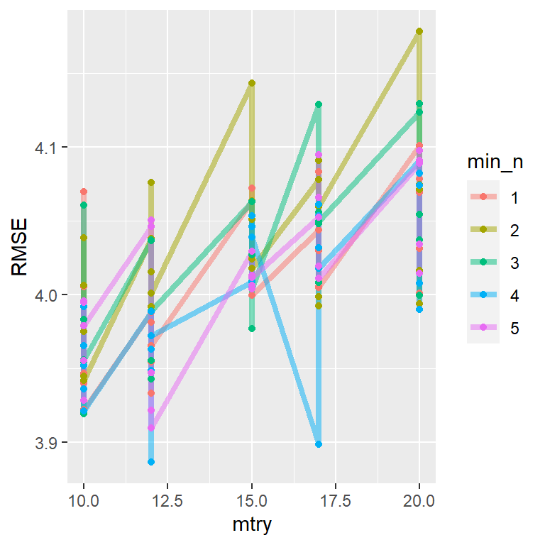
Now we will fit the models with all the possible parameter values on all our resampled (cv.fold) datasets. tune_grid() of tune package (installed with tidymodels) computes a set of performance metrics (e.g. accuracy or RMSE) for a pre-defined set of tuning parameters that correspond to a model or recipe across one or more resamples of the data.
We will use parallel processing to run RF model faster, since the different parts of the grid are independent. Let’s use grid = 20 to choose 20 grid points automatically.
tune_grid() computes a set of performance metrics (e.g. accuracy or RMSE) for a pre-defined set of tuning parameters that correspond to a model or recipe across one or more resamples of the data.
Random Forest Model Specification (regression)

Main Arguments:
  mtry = 12
  trees = 60
  min_n = 4

Computational engine: ranger
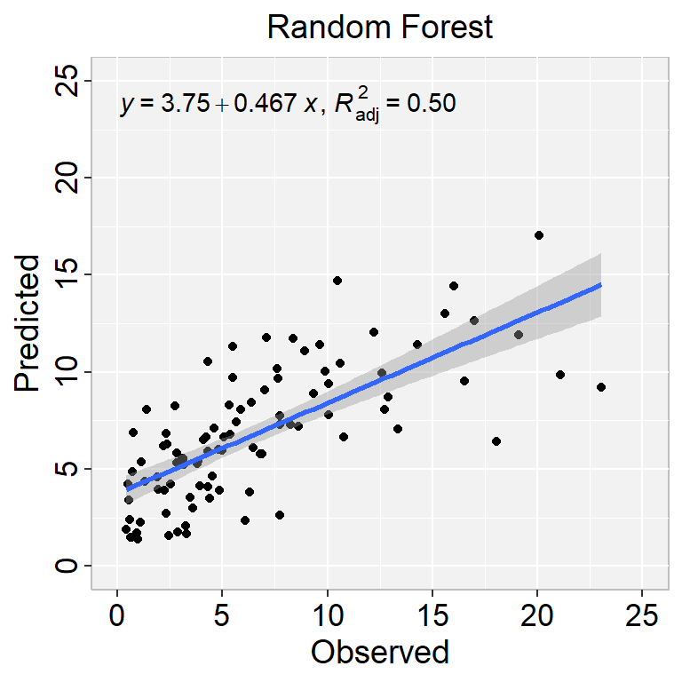
We can either fit final_tree to training data using fit() or to the testing/training split using last_fit(), which will give us some other results along with the fitted output.
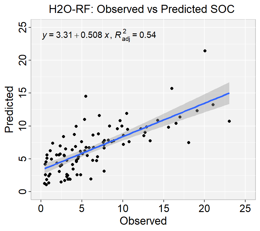
In h20, RF is known as Distributed Random Forest (DRF) which is the parallel implementation of the Random Forest algorithm. In DRF, each tree is trained on a random subset of the rows and columns of the training data. This randomness helps to reduce overfitting and improve the accuracy and robustness of the model. The predictions of the individual trees are then aggregated to make a final prediction.
DRF also provides various hyperparameters that can be tuned to optimize the performance of the model, including the number of trees, the depth of the trees, and the sampling rate for each tree. The algorithm also supports automatic hyperparameter tuning using grid search or random search.
Overall, DRF in H2O provides a powerful and scalable tool for building accurate and robust predictive models on large datasets. By distributing the computation across a cluster of machines, DRF can handle datasets that would be too large to process on a single machine, making it a valuable tool for big data applications.
Fit RF model without grid Search
First we will fit a DRF model with limited number fixed hyperparameters.
H2O is not running yet, starting it now...

Note:  In case of errors look at the following log files:
    C:\Users\zahmed2\AppData\Local\Temp\1\RtmpM3w6dT\file47102980317/h2o_zahmed2_started_from_r.out
    C:\Users\zahmed2\AppData\Local\Temp\1\RtmpM3w6dT\file4710548d7967/h2o_zahmed2_started_from_r.err


Starting H2O JVM and connecting:  Connection successful!

R is connected to the H2O cluster:
    H2O cluster uptime:         3 seconds 241 milliseconds
    H2O cluster timezone:       America/New_York
    H2O data parsing timezone:  UTC
    H2O cluster version:        3.40.0.4
    H2O cluster version age:    3 months and 23 days
    H2O cluster name:           H2O_started_from_R_zahmed2_qtu738
    H2O cluster total nodes:    1
    H2O cluster total memory:   198.00 GB
    H2O cluster total cores:    40
    H2O cluster allowed cores:  40
    H2O cluster healthy:        TRUE
    H2O Connection ip:          localhost
    H2O Connection port:        54321
    H2O Connection proxy:       NA
    H2O Internal Security:      FALSE
    R Version:                  R version 4.3.1 (2023-06-16 ucrt)
Code
#disable progress bar for RMarkdownh2o.no_progress() # Optional: remove anything from previous sessionh2o.removeAll()
rf_h2o <-h2o.randomForest( ## h2o.randomForest functiontraining_frame = h_train, ## the H2O frame for training# validation_frame = valid, ## the H2O frame for validation (not required)x=x, ## the predictor columns, by column indexy=y, ## the target index (what we are predicting)model_id ="RF_MODEL_IDs", ## name the model in H2O## not required, but helps use Flowntrees =200, ## use a maximum of 200 trees to create the## random forest model. The default is 50.## We will use 200 because it will let ## the early stopping criteria decide when## the random forest is sufficiently accuratemax_depth =25, ## Maximum tree depth (0 for unlimited). ## Defaults to 20.sample_rate =0.8, ## Row sample rate per tree (from 0.0 to 1.0) ## Defaults to 0.632.stopping_rounds =2, ## Stop fitting new trees when the 2-tree## average is within 0.001 (default) of ## the prior two 2-tree averages.stopping_metric ="RMSE", ## Metric to use for early stopping#score_each_iteration = TRUE, ## Predict against training and validation for## each tree. Default will skip several.nfolds =10, ## umber of folds for K-fold cross-validation ## (0 to disable or >= 2). Defaults to 0.keep_cross_validation_models =TRUE, ## logical. Whether to keep the cross-validation models. ## Defaults to TRUE.seed =1000000) ## Set the random seed so that this can be reproduced
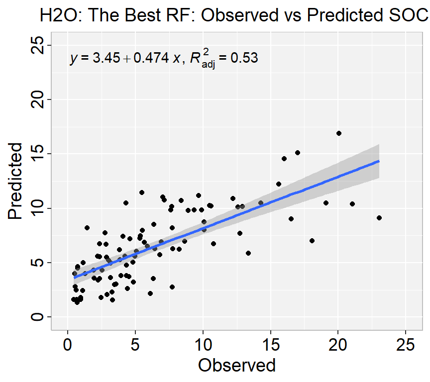
H2O Grid Search is a hyperparameter optimization technique used in the H2O machine learning framework. It involves a systematic search through a specified subset of hyperparameters of a machine learning model to find the optimal combination of hyperparameters that maximizes the performance metric of interest, such as RMSE or AUC.
In a grid search, a set of hyperparameters is defined, and a range of values is specified for each hyperparameter. The grid search algorithm then systematically evaluates all possible combinations of hyperparameter values, training and evaluating a model for each combination, and selecting the combination that performs the best on the validation set.
H2O Grid Search can be used with various machine learning models, including generalized linear models, random forest, gradient boosting machines, and deep learning models. It can help improve the performance of machine learning models by fine-tuning their hyperparameters and reducing overfitting.
H2O supports two types of grid search – traditional (or “cartesian”) grid search and random grid search. In a cartesian grid search, users specify a set of values for each hyperparameter that they want to search over, and H2O will train a model for every combination of the hyperparameter values. This means that if you have three hyperparameters and you specify 5, 10 and 2 values for each, your grid will contain a total of 5102 = 100 models.
Define RF Hyper-parameters
Code
RF_hyper_params <-list(ntrees =seq(10, 500, by =20), # number of treesmtries =seq(10, 40, by =10), # Number of variables randomly sampled as candidates at each split.max_depth =seq(20, 40, by =5), # Maximum tree depth (0 for unlimited). Defaults to 20.min_rows =seq(1, 5, by =1), # Fewest allowed (weighted) observations in a leaf. sample_rate =c(0.5, 0.6, 0.7, 0.8, 0.9)) # Row sample rate per tree (from 0.0 to 1.0) Defaults to 0.632.RF_hyper_params
search_criteria is a parameter that can be used to specify the stopping criteria for a grid search or a random grid search. By setting the search_criteria parameter, you can control the runtime and complexity of the grid search, and avoid overfitting by early stopping based on the validation metric.
search_criteria is a dictionary that contains one or more of the following parameters:
strategy: The search strategy to use, either “Cartesian” or “RandomDiscrete”. The default is “Cartesian”.
max_models: The maximum number of models to build. The default is NULL, which means to build all possible models.
max_runtime_secs: The maximum amount of time in seconds that the grid search can run. The default is NULL, which means to run until the other stopping criteria are met.
stopping_rounds: The number of consecutive builds without an improvement in the validation metric that triggers early stopping. The default is 0, which means to disable early stopping.
stopping_tolerance: The relative tolerance for the metric-based stopping criterion. The default is 0.001.
stopping_metric: The metric to use for the metric-based stopping criterion. The default is “AUTO”, which means to use the default metric for the specified problem type.
For example, to specify a maximum of 20 models to build and a maximum runtime of 600 seconds for a grid search, you can set the search_criteria parameter as follows:
RandomDiscrete grid search involves randomly sampling hyperparameters from a predefined set of discrete values and evaluating the performance of the model with each combination of hyperparameters.
This method is useful when the search space for hyperparameters is large and discrete, meaning that the values are distinct and finite. In contrast to a regular grid search, which evaluates all possible combinations of hyperparameters, a random search selects a random subset of hyperparameters to evaluate.
The advantage of using RandomDiscrete grid search is that it can be more efficient than a regular grid search, especially when many of the hyperparameters are not critical to the performance of the model. It can also help to prevent overfitting, as it encourages the exploration of a wider range of hyperparameters.
RF Grid Search
h2o.grid() provides a set of functions to launch a grid search and get its results:
# Get Model IDRF_get_grid <-h2o.getGrid("RF_grid_IDs",sort_by="RMSE",decreasing=F)# Get the best RF modelbest_RF <-h2o.getModel(RF_get_grid@model_ids[[1]])best_RF
Model explainability refers to the ability to understand and interpret the decisions made by a machine learning model. In other words, it is the ability to explain how a model arrives at its predictions or classifications.
Explainability is particularly important in applications where decisions made by the model have significant real-world consequences, such as in healthcare, finance, and legal fields. It is also important for regulatory compliance, where models must be auditable and transparent.
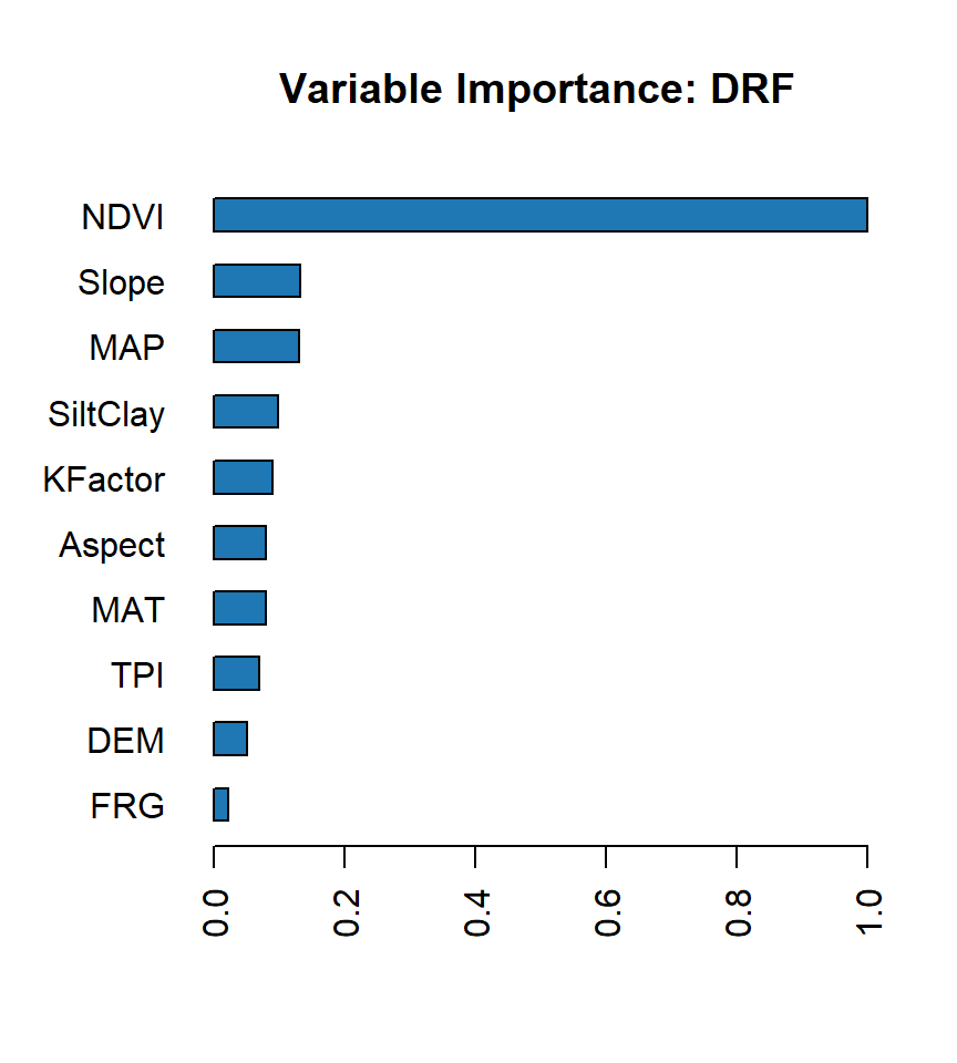
The h2o.explain() function generates a list of explanations – individual units of explanation such as a Partial Dependence plot or a Variable Importance plot. Most of the explanations are visual – these plots can also be created by individual utility functions outside the h2o.explain() function.
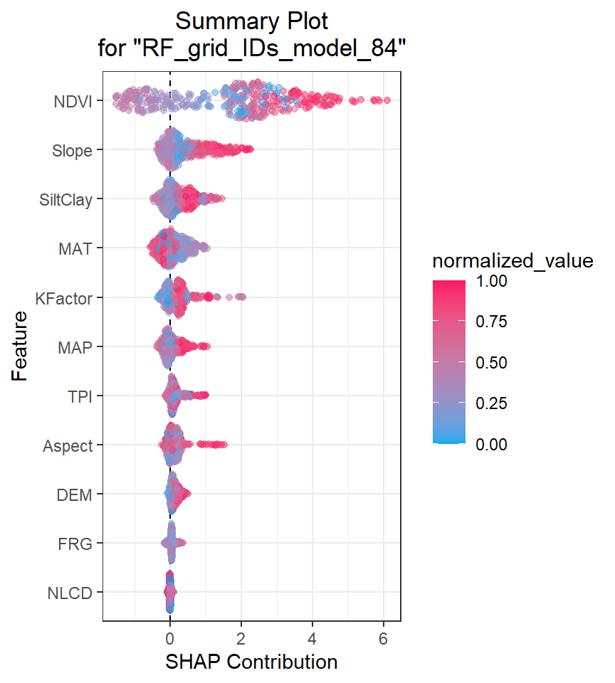
SHAP (SHapley Additive exPlanations) values are a method for explaining the output of any machine learning model. SHAP values provide a way to attribute the prediction of an individual feature to its contribution to the final prediction, taking into account the interaction with other features in the model.
SHAP values are based on the Shapley value from cooperative game theory, which attributes a value to each player in a game based on their contribution to the game’s outcome. In the context of machine learning, the “players” are the input features of the model, and the “game” is the prediction made by the model.
The SHAP value for a particular feature is calculated by comparing the model’s prediction for a specific data point with and without that feature’s value included. This comparison is done for all possible subsets of features, and the contributions of each feature are averaged using the Shapley value formula.
The resulting SHAP values represent the contribution of each feature to the final prediction, with positive values indicating a positive impact on the prediction and negative values indicating a negative impact.
SHAP values can be used to provide insights into how a model is making its predictions and to identify which features are most important for a particular prediction. They can also be used to identify bias in a model and to ensure that the model is making predictions fairly and transparently.
H2O implements TreeSHAP which when the features are correlated, can increase contribution of a feature that had no influence on the prediction.
Code
h2o.shap_summary_plot(best_RF, h_train)
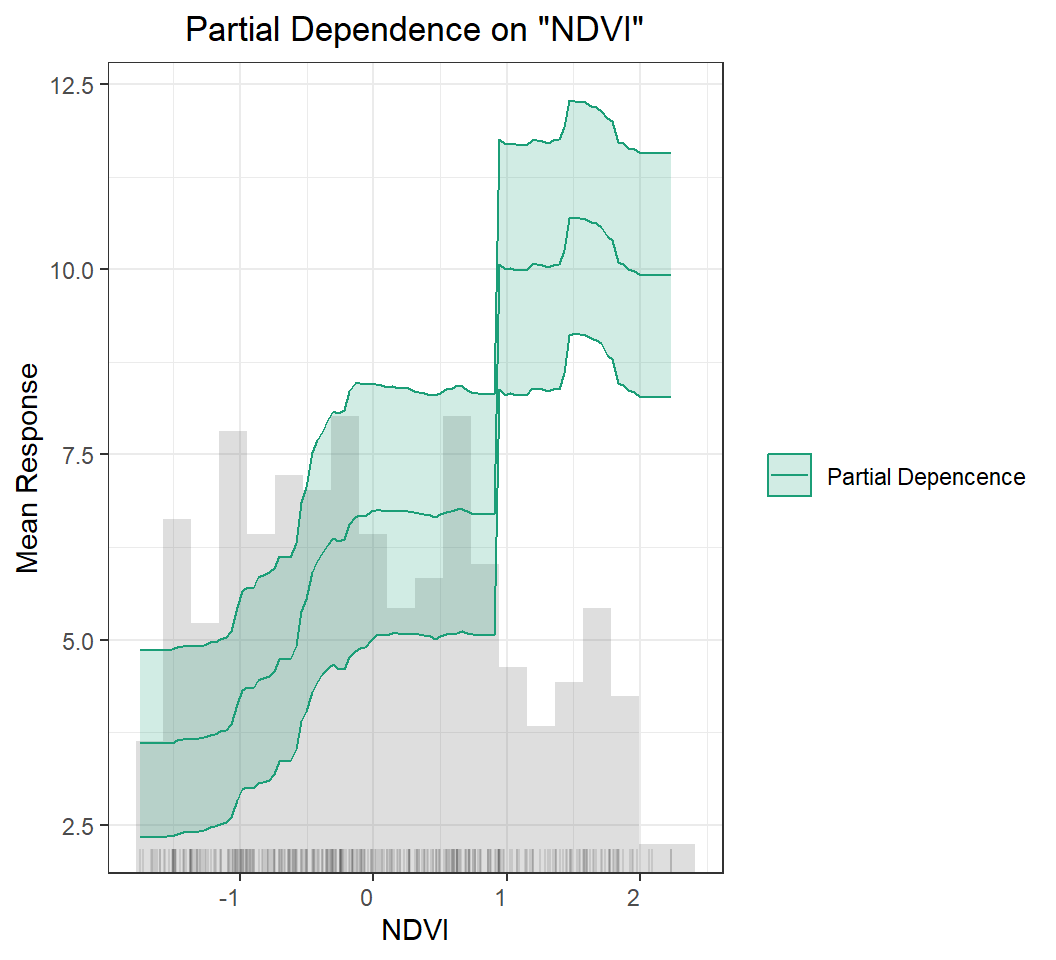
Partial Dependence (PD) Plots
A partial dependence plot (PDP) is a graphical tool for understanding the relationship between a particular input feature and the output of a machine learning model.
A PDP shows the marginal effect of a single feature on the predicted outcome while holding all other features at a fixed value or their average value. The PDP can help to visualize the shape and direction of the relationship between the feature and the output, and can also help to identify any non-linearities or interactions between the feature and other features in the model.
To create a PDP, the value of the feature of interest is varied over its range, and the model’s predicted output is recorded for each value. The resulting data is then plotted on a graph, with the feature’s value on the x-axis and the predicted output on the y-axis.
PDPs can be used to gain insights into how a model is making its predictions and to identify which features are most important for the model’s output. They can also be used to identify potential biases in the model or to detect interactions between features that may be difficult to detect using other methods.
Code
h2o.pd_multi_plot(best_RF, h_train, "NDVI")
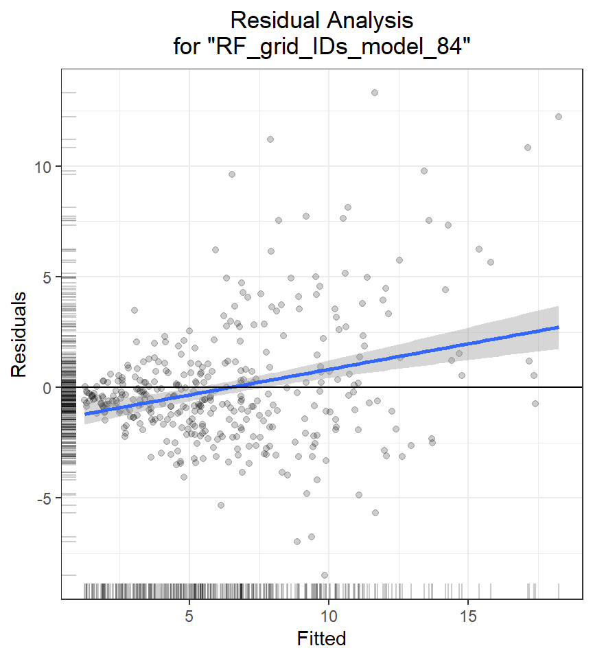
Residual Analysis
Residual Analysis plots the fitted values vs residuals on a test dataset. Ideally, residuals should be randomly distributed. Patterns in this plot can indicate potential problems with the model selection, e.g., using simpler model than necessary, not accounting for heteroscedasticity, autocorrelation, etc. Note that if you see “striped” lines of residuals, that is an artifact of having an integer valued (vs a real valued) response variable
Code
h2o.residual_analysis_plot(best_RF, h_train)
Code
# remove all objectrm(list =ls())
Exercise
Create a R-Markdown documents (name homework_13.rmd) in this project and do all Tasks using the data shown below.
Submit all codes and output as a HTML document (homework_13.html) before class of next week.
[{fig-align="right" width="176" height="64"}](https://github.com/zia207/r-colab/blob/main/random_forest.ipynb)# Random Forest (RF) {.unnumbered}Random Forest (RF) is a tree-based machine learning algorithm that is used for classification, regression and other tasks in data analysis. It is a popular and robust algorithm that builds multiple decision trees and combines their predictions to make a final prediction. RF is a modification of Bagging (bootstrap aggregating) regression trees that builds a large collection of de-correlated trees and has become a very popular "out-of-the-box" learning algorithm that has low variance and higher predictive power than traditional bagging models.Each decision tree in the Random Forest is constructed by randomly selecting a subset of the available features and then building a tree based on those features. This process is repeated a specified number of times, resulting in multiple decision trees. When a new data point needs to be classified, each tree in the forest is used to make a prediction, and the final prediction is based on the most common prediction made by all the trees.Random Forest is a robust algorithm because it can handle large datasets with many features and is also resistant to overfitting, which can occur when a model is too complex and fits the training data too closely. Random Forest works by using ensemble learning, which means combining the predictions of multiple models to improve accuracy and reduce errors.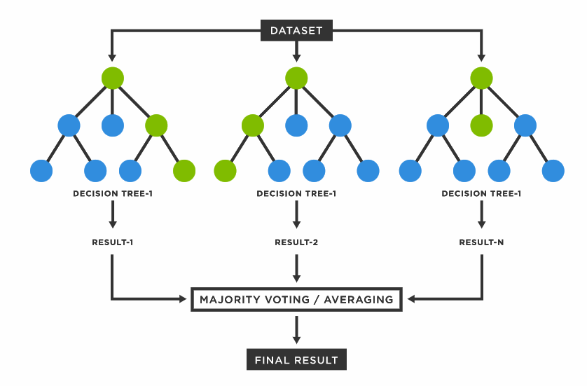{width="595"}Here is how Random Forest works step by step:1. Randomly select a subset of the dataset.2. Construct a decision tree on the selected subset of the dataset.3. Repeat steps 1 and 2 to construct multiple decision trees.4. Pass each input through all the decision trees and record their outputs.5. Determine the final output based on the majority vote (classification) or mean prediction (regression) of the decision trees.### DataIn this exercise we will use the following data set and use DEM, MAP, MAT, NAVI, NLCD, and FRG to fit an RF regression model.[gp_soil_data.csv](https://www.dropbox.com/s/9ikm5yct36oflei/gp_soil_data.csv?dl=0)```{r}#| warning: false#| error: falselibrary(tidyverse)# define data folderurlfile ="https://github.com//zia207/r-colab/raw/main/Data/USA/gp_soil_data.csv"mf<-read_csv(url(urlfile))# Create a data-framedf<-mf %>% dplyr::select(SOC, DEM, Slope, Aspect, TPI, KFactor, SiltClay, MAT, MAP,NDVI, NLCD, FRG)%>%glimpse()```## Random Forest with randomForest packageThe randomForest R package widely implements the random forest algorithm for building decision trees in machine learning. Random forests are an ensemble learning method that builds multiple decision trees and aggregates their predictions to make a final prediction. This can help to reduce overfitting and increase the accuracy of the model.The randomForest package in R provides a simple interface for building random forests. It allows the user to specify the number of trees to build, the number of variables to sample at each split, and other hyperparameters. The package also includes functions for visualizing the random forest model, as well as methods for predicting new data and assessing model performance.To get started with the randomForest package, you can install it from CRAN using the following code:> install.packages("randomForest)```{r}#| warning: false#| error: falselibrary(randomForest)```#### Split DataWe use **rsample** package, install with **tidymodels**, to split data into training (70%) and test data (30%) set with Stratified Random Sampling. initial_split() creates a single binary split of the data into a training set and testing set.::: callout-noteStratified random sampling is a technique for selecting a representative sample from a population, where the sample is chosen in a way that ensures that certain subgroups within the population are adequately represented in the sample.:::```{r }#| warning: false#| error: false##| fig.width: 4#| fig.height: 4library(tidymodels)set.seed(1245) # for reproducibilitysplit <-initial_split(df, prop =0.8, strata = SOC)train <- split %>%training()test <- split %>%testing()# Density plot all, train and test data ggplot()+geom_density(data = df, aes(SOC))+geom_density(data = train, aes(SOC), color ="green")+geom_density(data = test, aes(SOC), color ="red") +xlab("Soil Organic Carbon (kg/g)") +ylab("Density") ```#### Feature Scaling```{r}train[-c(1, 11,12)] =scale(train[-c(1,11,12)])test[-c(1, 11,12)] =scale(test[-c(1,11,12)])```#### Fit a random forest modelWe can fit a random forest model using the randomForest() function, which implements Breiman's random forest algorithm (based on Breiman and Cutler's original Fortran code) for classification and regression. It can also be used in unsupervised mode for assessing proximities among data points.```{r}#| warning: false#| error: falseset.seed(123) # for reproducibilityrf.fit <-randomForest(SOC ~ ., data=train, ntree=100, # Number of trees to growmtry =8, # Number of variables randomly sampled as candidates at each split#sampsize = 0.65 , # Size(s) of sample to draw#nodesize = 5, # Minimum size of terminal nodes#maxnode = 5, # maximum number of terminal nodeskeep.forest =TRUE, importance=TRUE)``````{r}rf.fit```#### Plot RF model```{r}#| warning: false#| error: false#| fig.width: 5#| fig.height: 4# Plotting modelplot(rf.fit)```#### Feature ImportanceFeature importance in Random Forest refers to a measure of the contribution of each feature to the accuracy of the model. The importance of each feature is determined by calculating the relative influence of each variable: whether that variable was selected to split on during the tree building process, and how much the squared error (over all trees) improved (decreased) as a result. The importance of a feature is the sum of the importance of that feature across all decision trees in the Random Forest.There are different methods to calculate feature importance in Random Forest. The most commonly used methods are:Gini Importance: It measures the total reduction of the Gini index, which is a measure of impurity, that is achieved by each feature. A higher reduction in the Gini index indicates a higher importance of the feature.Permutation Importance: It measures the decrease in the accuracy of the model when a feature is randomly permuted. A higher decrease in accuracy indicates a higher importance of the feature.Mean Decrease Impurity:In a Random Forest algorithm, node purity is a measure of how homogeneous the group of data points at a particular node is with respect to their target labels. The algorithm builds a decision tree by recursively splitting the data into smaller subsets based on the features and their values, with the aim of maximizing the node purity at each level.It measures the average reduction in impurity over all decision trees in the Random Forest when a feature is used to split a node. A higher reduction in impurity indicates a higher importance of the feature.In regression, the feature importance is calculated based on the mean decrease in impurity of the regression tree nodes or measures the variability of the target variable within the node.. The impurity measure used for regression is the mean squared error (MSE) instead of the Gini index used in classification.The importance of a feature is calculated by taking the total reduction in the MSE across all trees in the forest when the feature is used for splitting the nodes. A feature that reduces the MSE by a large amount is considered more important than a feature that reduces it by a smaller amount.The feature importance scores can be normalized so that they add up to one. This allows for easy comparison of the relative importance of different features.Once the feature importance is calculated, it can be used to select the most important features for the model or to interpret the model by understanding which features are driving the predictions.varImpPlot() function create dotchart of variable importance as measured by a Random Forest```{r}#| warning: false#| error: false#| fig.width: 8#| fig.height: 5# Variable importance plotvarImpPlot(rf.fit)```We can create a customize variable importance plot with ggplot2:```{r}#| warning: false#| error: false#| fig.width: 5#| fig.height: 4# Get variable importance from the model fitImpData <-as.data.frame(importance(rf.fit))ImpData$Var.Names <-row.names(ImpData)# Plot importanceggplot(ImpData, aes(y=`%IncMSE`, x=reorder(Var.Names, +`%IncMSE`))) +geom_segment( aes(x=reorder(Var.Names, +`%IncMSE`), xend=Var.Names, y=0, yend=`%IncMSE`), color="skyblue") +geom_point(aes(size = IncNodePurity), color="blue", alpha=0.8) +ylab('`%IncMSE`') +xlab('')+theme_bw() +theme(axis.line =element_line(colour ="black"),panel.grid.major =element_blank(),axis.text.y=element_text(size=12),axis.text.x =element_text(size=12),axis.title.x =element_text(size=12),axis.title.y =element_text(size=12))+coord_flip()+ggtitle("Random Forest Feature Importance")```An alternative approach is to use the vip package, which provides ggplot2 plots. vip also provides an additional measure of variable importance based on partial dependence measures and is a common variable importance plotting framework for many machine learning models```{r}#| warning: false#| error: false#| fig.width: 5#| fig.height: 4library(vip)vip(rf.fit)```#### Prediction```{r}test$SOC.pred =predict(rf.fit, newdata = test)``````{r}#| warning: false#| error: falselibrary(Matrix)RMSE<- Metrics::rmse(test$SOC, test$SOC.pred)RMSE``````{r}#| warning: false#| error: false#| fig.width: 4#| fig.height: 4library(ggpmisc)formula<-y~xggplot(test, aes(SOC,SOC.pred)) +geom_point() +geom_smooth(method ="lm")+stat_poly_eq(use_label(c("eq", "adj.R2")), formula = formula) +ggtitle("Random Forest") +xlab("Observed") +ylab("Predicted") +scale_x_continuous(limits=c(0,25), breaks=seq(0, 25, 5))+scale_y_continuous(limits=c(0,25), breaks=seq(0, 25, 5)) +# Flip the barstheme(panel.background =element_rect(fill ="grey95",colour ="gray75",size =0.5, linetype ="solid"),axis.line =element_line(colour ="grey"),plot.title =element_text(size =14, hjust =0.5),axis.title.x =element_text(size =14),axis.title.y =element_text(size =14),axis.text.x=element_text(size=13, colour="black"),axis.text.y=element_text(size=13,angle =90,vjust =0.5, hjust=0.5, colour='black'))```## Random Forest with tidymodelThe tidymodels provides a comprehensive framework for building, tuning, and evaluating RF model while following the principles of the tidyverse.#### Split data```{r}library(tidymodels)set.seed(1245) # for reproducibilitysplit <-initial_split(df, prop =0.8, strata = SOC)train <- split %>%training()test <- split %>%testing()# Set 10 fold cross-validation data set cv_folds <-vfold_cv(train, v =10)```#### Create RecipeA recipe is a description of the steps to be applied to a data set in order to prepare it for data analysis. Before training the model, we can use a recipe to do some pre-processing required by the model.```{r}#| warning: false#| error: false# load librarylibrary(tidymodels)# Create a reciperf_recipe <-recipe(SOC ~ ., data = train) %>%step_zv(all_predictors()) %>%step_dummy(all_nominal()) %>%step_normalize(all_numeric_predictors())```#### Specify tunable Hypermeters of Random ForestRandom Forest is an ensemble learning method that is highly flexible and has a large number of hyperparameters that can be tuned to optimize the performance of the model.Some of the most important hyperparameters of a Random Forest model are:1. Number of trees: The number of trees in the forest. Increasing the number of trees generally improves the performance of the model, but also increases the computation time.2. Maximum depth of the trees: The maximum depth of the trees in the forest. Deeper trees can capture more complex relationships in the data, but can also lead to overfitting.3. Minimum number of samples required to split a node: The minimum number of samples required to split an internal node in the tree. Increasing this parameter can help to reduce overfitting.4. Minimum number of samples required to be at a leaf node: The minimum number of samples required to be at a leaf node. Increasing this parameter can help to reduce overfitting.5. Maximum number of features to consider for each split: The maximum number of features to consider when searching for the best split at each node. Restricting the number of features can help to reduce overfitting and improve generalization.6. Bootstrap samples: Whether to use bootstrap samples when building trees. Bootstrap samples can help to reduce overfitting and improve generalization.7. Random state: A seed value that is used to initialize the random number generator. This ensures that the results of the model are reproducible.These hyperparameters can be tuned using various techniques, such as grid search or random search, to find the optimal combination for a particular dataset and problem.We will create a model specification for a random forest where we will tune tree (numbrr of tree), mtry (the number of predictors to sample at each split) and min_n (the number of observations needed to keep splitting nodes). Will will use [ranger](https://cran.r-project.org/web/packages/ranger/index.html) package that provides a fast implementation of the Random Forest algorithm for classification and regression problems. It is designed to handle large datasets with many features, and offers several features that make it a popular choice for machine learning tasks.> install.packages("ranger")```{r}#| warning: false#| error: falserf_model <-rand_forest(mtry =tune(),trees =tune(),min_n =tune() ) %>%set_mode("regression") %>%set_engine("ranger")rf_model```#### Define workflow```{r}#| warning: false#| error: falserf_wf <-workflow() %>%add_recipe(rf_recipe) %>%add_model(rf_model)```#### Define possible grid parameterWe use grid_regular() function of dials package (installed with tidymodesl) to create grids of tuning parameters```{r}#| warning: false#| error: falserf_grid <-grid_regular(trees(range =c(20, 100)),mtry(range =c(10, 20)),min_n(range =c(1, 5)),levels =5)rf_grid```#### Hyperparameters tunningNow we will fit the models with all the possible parameter values on all our resampled (cv.fold) datasets. tune_grid() of tune package (installed with tidymodels) computes a set of performance metrics (e.g. accuracy or RMSE) for a pre-defined set of tuning parameters that correspond to a model or recipe across one or more resamples of the data.We will use parallel processing to run RF model faster, since the different parts of the grid are independent. Let's use grid = 20 to choose 20 grid points automatically.tune_grid() computes a set of performance metrics (e.g. accuracy or RMSE) for a pre-defined set of tuning parameters that correspond to a model or recipe across one or more resamples of the data.```{r}#| warning: false#| error: false#| doParallel::registerDoParallel()set.seed(345)rf_tune <-tune_grid( rf_wf,resamples = cv_folds,grid = rf_grid, )rf_tune``````{r}collect_metrics(rf_tune)```We can plot RMSE:```{r}#| fig.width: 4#| fig.height: 4rf_tune %>%collect_metrics() %>%filter(.metric =="rmse") %>%mutate(min_n =factor(min_n)) %>%ggplot(aes(mtry, mean, color = min_n)) +geom_line(alpha =0.5, size =1.5) +geom_point() +labs(y ="RMSE")```#### The best RF model```{r}best_rmse <-select_best(rf_tune, "rmse")rf_final <-finalize_model( rf_model, best_rmse)rf_final```We can either fit final_tree to training data using fit() or to the testing/training split using last_fit(), which will give us some other results along with the fitted output.```{r}#| warning: false#| error: falsefinal_fit <-fit(rf_final, SOC ~ .,train)```#### Prediction```{r}test$SOC.pred =predict(final_fit,test)``````{r}#| warning: false#| error: falselibrary(Matrix)RMSE<- Metrics::rmse(test$SOC, test$SOC.pred$.pred)RMSE``````{r}#| warning: false#| error: false#| fig.width: 4#| fig.height: 4library(ggpmisc)formula<-y~xggplot(test, aes(SOC,SOC.pred$.pred)) +geom_point() +geom_smooth(method ="lm")+stat_poly_eq(use_label(c("eq", "adj.R2")), formula = formula) +ggtitle("Random Forest") +xlab("Observed") +ylab("Predicted") +scale_x_continuous(limits=c(0,25), breaks=seq(0, 25, 5))+scale_y_continuous(limits=c(0,25), breaks=seq(0, 25, 5)) +# Flip the barstheme(panel.background =element_rect(fill ="grey95",colour ="gray75",size =0.5, linetype ="solid"),axis.line =element_line(colour ="grey"),plot.title =element_text(size =14, hjust =0.5),axis.title.x =element_text(size =14),axis.title.y =element_text(size =14),axis.text.x=element_text(size=13, colour="black"),axis.text.y=element_text(size=13,angle =90,vjust =0.5, hjust=0.5, colour='black'))```#### Variable importance plotsvip() function can plot variable importance scores for the predictors in a model.> imstall.package("vip")```{r}#| warning: false#| error: false#| fig.width: 5.5#| fig.height: 6library(vip)rf_prep <-prep(rf_recipe)juiced <-juice(rf_prep)rf_final %>%set_engine("ranger", importance ="permutation") %>%fit(SOC ~ .,data =juice(rf_prep) ) %>%vip(geom ="point")```## Random Forest with h20In h20, RF is known as Distributed Random Forest (DRF) which is the parallel implementation of the Random Forest algorithm. In DRF, each tree is trained on a random subset of the rows and columns of the training data. This randomness helps to reduce overfitting and improve the accuracy and robustness of the model. The predictions of the individual trees are then aggregated to make a final prediction.DRF also provides various hyperparameters that can be tuned to optimize the performance of the model, including the number of trees, the depth of the trees, and the sampling rate for each tree. The algorithm also supports automatic hyperparameter tuning using grid search or random search.Overall, DRF in H2O provides a powerful and scalable tool for building accurate and robust predictive models on large datasets. By distributing the computation across a cluster of machines, DRF can handle datasets that would be too large to process on a single machine, making it a valuable tool for big data applications.### Fit RF model without grid SearchFirst we will fit a DRF model with limited number fixed hyperparameters.#### Convert to factor```{r}#| warning: false#| error: falsedf$NLCD <-as.factor(df$NLCD)df$FRG <-as.factor(df$FRG)```#### Data split```{r}#| warning: false#| error: falselibrary(tidymodels)set.seed(1245) # for reproducibilitysplit.df <-initial_split(df, prop =0.8, strata = SOC)train <- split.df %>%training()test <- split.df %>%testing()```#### Feature Scaling```{r}train[-c(1, 11,12)] =scale(train[-c(1,11,12)])test[-c(1, 11,12)] =scale(test[-c(1,11,12)])```#### Import h2o```{r}#| warning: false#| error: falselibrary(h2o)h2o.init(nthreads =-1, max_mem_size ="198g", enable_assertions =FALSE) #disable progress bar for RMarkdownh2o.no_progress() # Optional: remove anything from previous sessionh2o.removeAll() ```#### Import data to h2o cluster```{r}#| warning: false#| error: falseh_df=as.h2o(df)h_train =as.h2o(train)h_test =as.h2o(test)``````{r}CV.xy<-as.data.frame(h_train)test.xy<-as.data.frame(h_test)```#### Define response and predictors```{r}#| warning: false#| error: falsey <-"SOC"x <-setdiff(names(h_df), y)```#### Fit a RF Model```{r}#| warning: false#| error: falserf_h2o <-h2o.randomForest( ## h2o.randomForest functiontraining_frame = h_train, ## the H2O frame for training# validation_frame = valid, ## the H2O frame for validation (not required)x=x, ## the predictor columns, by column indexy=y, ## the target index (what we are predicting)model_id ="RF_MODEL_IDs", ## name the model in H2O## not required, but helps use Flowntrees =200, ## use a maximum of 200 trees to create the## random forest model. The default is 50.## We will use 200 because it will let ## the early stopping criteria decide when## the random forest is sufficiently accuratemax_depth =25, ## Maximum tree depth (0 for unlimited). ## Defaults to 20.sample_rate =0.8, ## Row sample rate per tree (from 0.0 to 1.0) ## Defaults to 0.632.stopping_rounds =2, ## Stop fitting new trees when the 2-tree## average is within 0.001 (default) of ## the prior two 2-tree averages.stopping_metric ="RMSE", ## Metric to use for early stopping#score_each_iteration = TRUE, ## Predict against training and validation for## each tree. Default will skip several.nfolds =10, ## umber of folds for K-fold cross-validation ## (0 to disable or >= 2). Defaults to 0.keep_cross_validation_models =TRUE, ## logical. Whether to keep the cross-validation models. ## Defaults to TRUE.seed =1000000) ## Set the random seed so that this can be reproduced``````{r}summary(rf_h2o)```#### Model performance```{r}# training performanceh2o.performance(rf_h2o, h_train)# CV-performanceh2o.performance(rf_h2o, xval=TRUE)# test performanceh2o.performance(rf_h2o, h_test)```##### Prediction```{r}pred.rf <-as.data.frame(h2o.predict(object = rf_h2o, newdata = h_test))test_data<-as.data.frame(h_test)test_data$RF_SOC<-pred.rf$predict ```We can plot observed and predicted values with fitted regression line with ggplot2```{r}#| warning: false#| error: false#| fig.width: 4.5#| fig.height: 4library(ggpmisc)formula<-y~xggplot(test_data, aes(SOC,RF_SOC)) +geom_point() +geom_smooth(method ="lm")+stat_poly_eq(use_label(c("eq", "adj.R2")), formula = formula) +ggtitle("H2O-RF: Observed vs Predicted SOC ") +xlab("Observed") +ylab("Predicted") +scale_x_continuous(limits=c(0,25), breaks=seq(0, 25, 5))+scale_y_continuous(limits=c(0,25), breaks=seq(0, 25, 5)) +# Flip the barstheme(panel.background =element_rect(fill ="grey95",colour ="gray75",size =0.5, linetype ="solid"),axis.line =element_line(colour ="grey"),plot.title =element_text(size =14, hjust =0.5),axis.title.x =element_text(size =14),axis.title.y =element_text(size =14),axis.text.x=element_text(size=13, colour="black"),axis.text.y=element_text(size=13,angle =90,vjust =0.5, hjust=0.5, colour='black'))```### Fit the Best RF model with hyperparameter tunningH2O Grid Search is a hyperparameter optimization technique used in the H2O machine learning framework. It involves a systematic search through a specified subset of hyperparameters of a machine learning model to find the optimal combination of hyperparameters that maximizes the performance metric of interest, such as RMSE or AUC.In a grid search, a set of hyperparameters is defined, and a range of values is specified for each hyperparameter. The grid search algorithm then systematically evaluates all possible combinations of hyperparameter values, training and evaluating a model for each combination, and selecting the combination that performs the best on the validation set.H2O Grid Search can be used with various machine learning models, including generalized linear models, random forest, gradient boosting machines, and deep learning models. It can help improve the performance of machine learning models by fine-tuning their hyperparameters and reducing overfitting.H2O supports two types of grid search -- traditional (or "cartesian") grid search and random grid search. In a cartesian grid search, users specify a set of values for each hyperparameter that they want to search over, and H2O will train a model for every combination of the hyperparameter values. This means that if you have three hyperparameters and you specify 5, 10 and 2 values for each, your grid will contain a total of 5*10*2 = 100 models.#### Define RF Hyper-parameters```{r}#| warning: false#| error: falseRF_hyper_params <-list(ntrees =seq(10, 500, by =20), # number of treesmtries =seq(10, 40, by =10), # Number of variables randomly sampled as candidates at each split.max_depth =seq(20, 40, by =5), # Maximum tree depth (0 for unlimited). Defaults to 20.min_rows =seq(1, 5, by =1), # Fewest allowed (weighted) observations in a leaf. sample_rate =c(0.5, 0.6, 0.7, 0.8, 0.9)) # Row sample rate per tree (from 0.0 to 1.0) Defaults to 0.632.RF_hyper_params```#### RF Search Criteriasearch_criteria is a parameter that can be used to specify the stopping criteria for a grid search or a random grid search. By setting the search_criteria parameter, you can control the runtime and complexity of the grid search, and avoid overfitting by early stopping based on the validation metric.search_criteria is a dictionary that contains one or more of the following parameters:**strategy**: The search strategy to use, either "Cartesian" or "RandomDiscrete". The default is "Cartesian".**max_models**: The maximum number of models to build. The default is NULL, which means to build all possible models.**max_runtime_secs**: The maximum amount of time in seconds that the grid search can run. The default is NULL, which means to run until the other stopping criteria are met.**stopping_rounds**: The number of consecutive builds without an improvement in the validation metric that triggers early stopping. The default is 0, which means to disable early stopping.**stopping_tolerance**: The relative tolerance for the metric-based stopping criterion. The default is 0.001.**stopping_metric**: The metric to use for the metric-based stopping criterion. The default is "AUTO", which means to use the default metric for the specified problem type.For example, to specify a maximum of 20 models to build and a maximum runtime of 600 seconds for a grid search, you can set the search_criteria parameter as follows:```{r}#| warning: false#| error: false# RF_search_criteria <-list(strategy ="RandomDiscrete", max_models =200,max_runtime_secs =900,stopping_tolerance =0.001,stopping_rounds =2,seed =42)```::: callout-noteRandomDiscrete grid search involves randomly sampling hyperparameters from a predefined set of discrete values and evaluating the performance of the model with each combination of hyperparameters.This method is useful when the search space for hyperparameters is large and discrete, meaning that the values are distinct and finite. In contrast to a regular grid search, which evaluates all possible combinations of hyperparameters, a random search selects a random subset of hyperparameters to evaluate.The advantage of using RandomDiscrete grid search is that it can be more efficient than a regular grid search, especially when many of the hyperparameters are not critical to the performance of the model. It can also help to prevent overfitting, as it encourages the exploration of a wider range of hyperparameters.:::#### RF Grid Searchh2o.grid() provides a set of functions to launch a grid search and get its results:```{r}#| warning: false#| error: falserf_grid <-h2o.grid(algorithm="randomForest",grid_id ="RF_grid_IDs",x = x,y = y,training_frame = h_train,#validation_frame = h_valid,stopping_metric ="RMSE",#fold_assignment ="Stratified",nfolds=10,keep_cross_validation_predictions =TRUE,keep_cross_validation_models =TRUE,hyper_params = RF_hyper_params,search_criteria = RF_search_criteria,seed =42)```#### Best RF Model```{r}#| warning: false#| error: false# number RFlength(rf_grid@model_ids)# Get Model IDRF_get_grid <-h2o.getGrid("RF_grid_IDs",sort_by="RMSE",decreasing=F)# Get the best RF modelbest_RF <-h2o.getModel(RF_get_grid@model_ids[[1]])best_RF```##### Model performance```{r}# training performanceh2o.performance(best_RF, h_train)# CV-performanceh2o.performance(best_RF, xval=TRUE)# test performanceh2o.performance(best_RF, h_test)```#### Prediction```{r message=FALSE, warning=FALSE}# test - predictiontest.pred.RF<-as.data.frame(h2o.predict(object = best_RF, newdata = h_test))test.xy$RF_SOC<-test.pred.RF$predict```We can plot observed and predicted values with fitted regression line with ggplot2```{r}#| warning: false#| error: false#| fig.width: 4.5#| fig.height: 4library(ggpmisc)formula<-y~xggplot(test.xy, aes(SOC,RF_SOC)) +geom_point() +geom_smooth(method ="lm")+stat_poly_eq(use_label(c("eq", "adj.R2")), formula = formula) +ggtitle("H2O: The Best RF: Observed vs Predicted SOC ") +xlab("Observed") +ylab("Predicted") +scale_x_continuous(limits=c(0,25), breaks=seq(0, 25, 5))+scale_y_continuous(limits=c(0,25), breaks=seq(0, 25, 5)) +# Flip the barstheme(panel.background =element_rect(fill ="grey95",colour ="gray75",size =0.5, linetype ="solid"),axis.line =element_line(colour ="grey"),plot.title =element_text(size =14, hjust =0.5),axis.title.x =element_text(size =14),axis.title.y =element_text(size =14),axis.text.x=element_text(size=13, colour="black"),axis.text.y=element_text(size=13,angle =90,vjust =0.5, hjust=0.5, colour='black'))```#### Model ExplainabilityModel explainability refers to the ability to understand and interpret the decisions made by a machine learning model. In other words, it is the ability to explain how a model arrives at its predictions or classifications.Explainability is particularly important in applications where decisions made by the model have significant real-world consequences, such as in healthcare, finance, and legal fields. It is also important for regulatory compliance, where models must be auditable and transparent.The h2o.explain() function generates a list of explanations -- individual units of explanation such as a Partial Dependence plot or a Variable Importance plot. Most of the explanations are visual -- these plots can also be created by individual utility functions outside the h2o.explain() function.##### Retrieve the variable importance.```{r}#| warning: false#| error: falseh2o.varimp(best_RF)```#### Variable Importance Plot```{r}#| warning: false#| error: false#| fig.width: 4.5#| fig.height: 5h2o.varimp_plot(best_RF)```#### SHAP Local ExplanationSHAP (SHapley Additive exPlanations) values are a method for explaining the output of any machine learning model. SHAP values provide a way to attribute the prediction of an individual feature to its contribution to the final prediction, taking into account the interaction with other features in the model.SHAP values are based on the Shapley value from cooperative game theory, which attributes a value to each player in a game based on their contribution to the game's outcome. In the context of machine learning, the "players" are the input features of the model, and the "game" is the prediction made by the model.The SHAP value for a particular feature is calculated by comparing the model's prediction for a specific data point with and without that feature's value included. This comparison is done for all possible subsets of features, and the contributions of each feature are averaged using the Shapley value formula.The resulting SHAP values represent the contribution of each feature to the final prediction, with positive values indicating a positive impact on the prediction and negative values indicating a negative impact.SHAP values can be used to provide insights into how a model is making its predictions and to identify which features are most important for a particular prediction. They can also be used to identify bias in a model and to ensure that the model is making predictions fairly and transparently.H2O implements TreeSHAP which when the features are correlated, can increase contribution of a feature that had no influence on the prediction.```{r}#| warning: false#| error: false#| fig.width: 4.5#| fig.height: 5h2o.shap_summary_plot(best_RF, h_train)```#### Partial Dependence (PD) PlotsA partial dependence plot (PDP) is a graphical tool for understanding the relationship between a particular input feature and the output of a machine learning model.A PDP shows the marginal effect of a single feature on the predicted outcome while holding all other features at a fixed value or their average value. The PDP can help to visualize the shape and direction of the relationship between the feature and the output, and can also help to identify any non-linearities or interactions between the feature and other features in the model.To create a PDP, the value of the feature of interest is varied over its range, and the model's predicted output is recorded for each value. The resulting data is then plotted on a graph, with the feature's value on the x-axis and the predicted output on the y-axis.PDPs can be used to gain insights into how a model is making its predictions and to identify which features are most important for the model's output. They can also be used to identify potential biases in the model or to detect interactions between features that may be difficult to detect using other methods.```{r}#| warning: false#| error: false#| fig.width: 5.5#| fig.height: 5h2o.pd_multi_plot(best_RF, h_train, "NDVI")```##### Residual AnalysisResidual Analysis plots the fitted values vs residuals on a test dataset. Ideally, residuals should be randomly distributed. Patterns in this plot can indicate potential problems with the model selection, e.g., using simpler model than necessary, not accounting for heteroscedasticity, autocorrelation, etc. Note that if you see "striped" lines of residuals, that is an artifact of having an integer valued (vs a real valued) response variable```{r}#| warning: false#| error: false#| fig.width: 4.5#| fig.height: 5h2o.residual_analysis_plot(best_RF, h_train)``````{r}# remove all objectrm(list =ls())```### Exercise1. Create a R-Markdown documents (name homework_13.rmd) in this project and do all Tasks using the data shown below.2. Submit all codes and output as a HTML document (homework_13.html) before class of next week.#### Required R-Packagetidyverse, caret, Metrics, tidymodels, vip#### Data1. [bd_soil_update.csv](https://www.dropbox.com/s/jtzycm4kg3lngu3/bd_soil_update.csv?dl=0)Download the data and save in your project directory. Use read_csv to load the data in your R-session. For example:> mf\<-read_csv("bd_soil_update.csv")#### Tasks1. Create a data-frame for random forest model of SOC with following variables for Rajshahi Division: First use filter() to select data from Rajshai division and then use select() functions to create data-frame with following variables: SOM, DEM, NDVI, NDFI,2. Fit and show the model performance of a RF model with using randomForest and h20 packages.3. Find the best RF model with grid search using tidymodels and h2o and show all steps as shown in the tutorials,### Further Reading1. [Random Forest in R](https://www.r-bloggers.com/2021/04/random-forest-in-r/)2. [Tuning random forest hyperparameters with #TidyTuesday trees data](https://juliasilge.com/blog/sf-trees-random-tuning/)3. [GBM_RandomForest_Example.R](https://github.com/h2oai/h2o-tutorials/blob/master/tutorials/gbm-randomforest/GBM_RandomForest_Example.R)4. [Training and Turning Parameters for Random Forest Using h2o Package](https://rpubs.com/chidungkt/449576)### YouTube Video1. Visual Guide to Random Forest{{< video https://www.youtube.com/watch?v=cIbj0WuK41w&t=224s >}}Source: [Econoscent](https://www.youtube.com/@Econoscent)2. StatQuest: Random Forests Part 1 - Building, Using and Evaluating{{< video https://www.youtube.com/watch?v=J4Wdy0Wc_xQ >}}Source: [StatQuest with Josh Starme](https://www.youtube.com/@statquest)