Geometric Operations on Vector Data

Geometric operations on vector data in the context of spatial analysis involve manipulating and analyzing the shapes and relationships between different geographic features such as points, lines, and polygons. These operations help you extract meaningful insights from spatial data. Here are some common geometric operations you can perform on vector data using the sf package in R or similar geospatial libraries:

Buffering: Creating a buffer around points, lines, or polygons. Buffers represent an area a specified distance from the original features. Useful for proximity analysis, such as identifying points within a certain distance of a feature.
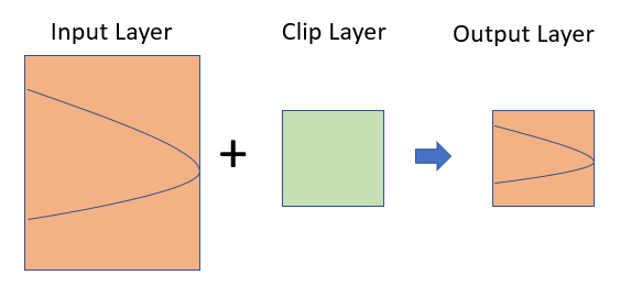
Clipping: Selecting a subset of features within the boundary of another feature. Useful for extracting relevant features within a specific area of interest.
Intersection: Finding the shared area or overlapping region between two or more features. Useful for determining areas of overlap or common boundaries.
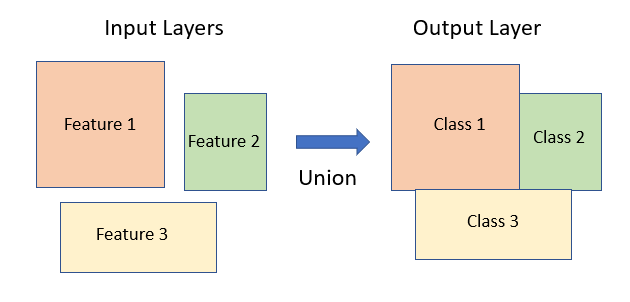
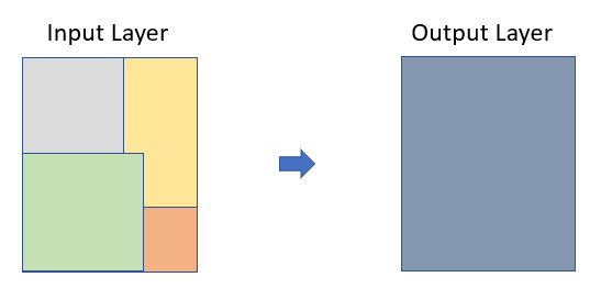
Union: Combining overlapping or adjacent features into a single feature. Useful in for merging features or creating new spatial units.
Difference: Finding the portion of one feature that does not overlap with another feature. Helpful in identifying the non-shared areas between features.
Dissolve: Aggregating features that share a with attribute value to create a single, multipart feature. Useful for creating regional summaries or simplifying datasets.
Splitting: Dividing a feature into two or more features using a line or polygon. Useful for partitioning areas or lines based on specific criteria.
Convex Hull: Creating the smallest convex polygon that encloses a set of points. Useful for analyzing the extent of point distributions.
Voronoi Diagrams: Dividing a space into regions based on the proximity to a set of points. Useful for spatial analysis and allocation.
Centroid and Centroid-based Operations: Calculating the centroid (center of mass) of a polygon or line. Useful for labeling or spatial analysis.
Simplification: Reducing the complexity of a geometry while preserving its essential shape. Useful for generalization and improving processing efficiency.
Affine Transformations: Applying transformations such as translation, rotation, scaling, and shearing to a geometry. Useful for geometric adjustments.

These operations are essential for various spatial analyses, including urban planning, environmental modeling, transportation analysis, and more. When performing these operations, make sure to consider the projection and coordinate system of your data to ensure accurate and meaningful results. The sf package in R provides a wide range of functions to perform these geometric operations, and similar capabilities can be found in other geospatial libraries and software.

Load Packages

Code

library(sf)       
library (rgdal)     
library (raster)    
library(tidyverse)
library(rgeos)
library(maptools)
library(terra)

Data

In this exercise we use following data set:

Spatial polygon of the district of Bangladesh (bd_district_BTM.shp)
Spatial polygon of the division of Bangladesh (bd_division_BTM.shp)
Spatial point data of soil sampling location under Rajshahi Division of Bangladesh (raj_soil_data.BTM.shp)
Road data of Rajshahi Division of Bangladesh (raj_road_BTM.shp)
Spatial polygon of Sundarban area (sundarban_BTM.shp)

Spatial Clipping

Clipping spatial data involves selecting a subset of spatial features (points, lines, polygons) from one dataset that are located within the boundaries of another dataset. This operation is commonly used to extract relevant geographic features or study areas from larger spatial datasets. For vector data, it involves removing unwanted features outside of an area of interest. For example, you might want to do some geospatial modeling covering a area in Rajshai Division in Bangladesh, but we may have data for the enitre country, in this case you need to apply clipping function to remove area outside of the New York State. It acts like a cookie cutter to cut out a piece of one feature class using one or more of the features in another feature class.

In R, you can do this several ways with different R packages. The st_intersection() function of the sf package is used to compute the geometric intersection of two or more spatial objects, resulting in a new spatial object that represents the shared area or overlapping region between the input geometries. Base R subsetting methods include the operator [ and the function subset() or dplyr subsetting functions filter() on vector attribute of “sf” objects do similar task. can be apply on attribute

In this exercise, we will clip out other districts from district shape files, expect our area of interest (for example Rajshai Division). First we will will rename “ADM1_EN” to “DIV_Name” and then filter out the Rajshahi division.

For reading ESRI shape file, we can use either readOGR() of rgdal or shapefile of raster packages to read shape file as SP objects from your local drive.

Code

# Define data folder
dataFolder<-"G:\\My Drive\\Data\\Bangladesh\\"
# if data in working directory
bd.div.sp<-raster::shapefile(paste0(dataFolder, "/Shapefiles/bd_division_BTM.shp"))  
bd.dist.sp<-raster::shapefile(paste0(dataFolder, "/Shapefiles/bd_district_BTM.shp"))

You may also use st_read() from sf package to load shapefile directly as SF objects from my github using GDAL Virtual File Systems (vsicurl).

Code

# define file from my github
bd.div.st = sf::st_read("/vsicurl/https://github.com//zia207/r-colab/raw/main/Data/Bangladesh//Shapefiles/bd_division_BTM.shp")

Reading layer `bd_division_BTM' from data source 
  `/vsicurl/https://github.com//zia207/r-colab/raw/main/Data/Bangladesh//Shapefiles/bd_division_BTM.shp' 
  using driver `ESRI Shapefile'
Simple feature collection with 8 features and 12 fields
Geometry type: MULTIPOLYGON
Dimension:     XY
Bounding box:  xmin: 298487.8 ymin: 278578.1 xmax: 778101.8 ymax: 946939.2
Projected CRS: +proj=tmerc +lat_0=0 +lon_0=90 +k=0.9996 +x_0=500000 +y_0=-2000000 +datum=WGS84 +units=m +no_defs

Code

bd.dist.st = sf::st_read("/vsicurl/https://github.com//zia207/r-colab/raw/main/Data/Bangladesh//Shapefiles//bd_district_BTM.shp")

Reading layer `bd_district_BTM' from data source 
  `/vsicurl/https://github.com//zia207/r-colab/raw/main/Data/Bangladesh//Shapefiles//bd_district_BTM.shp' 
  using driver `ESRI Shapefile'
Simple feature collection with 64 features and 14 fields
Geometry type: MULTIPOLYGON
Dimension:     XY
Bounding box:  xmin: 298487.8 ymin: 278578.1 xmax: 778101.8 ymax: 946939.2
Projected CRS: +proj=tmerc +lat_0=0 +lon_0=90 +k=0.9996 +x_0=500000 +y_0=-2000000 +datum=WGS84 +units=m +no_defs

Code

raj.div.st = bd.div.st %>%
  rename(DIV_Name = ADM1_EN) %>%
  filter(DIV_Name == "Rajshahi") %>%
  glimpse()

Rows: 1
Columns: 13
$ Shape_Leng <dbl> 8.410221
$ Shape_Area <dbl> 1.624856
$ DIV_Name   <chr> "Rajshahi"
$ ADM1_PCODE <chr> "BD50"
$ ADM1_REF   <chr> NA
$ ADM1ALT1EN <chr> NA
$ ADM1ALT2EN <chr> NA
$ ADM0_EN    <chr> "Bangladesh"
$ ADM0_PCODE <chr> "BD"
$ date       <chr> "2015/01/01"
$ validOn    <chr> "2020/11/13"
$ validTo    <chr> NA
$ geometry   <MULTIPOLYGON [m]> MULTIPOLYGON (((402152.5 79...

Then we will use st_intersection() to clip out all districts under Rajshai division from district shapefile

Code

raj.dist.st<-st_intersection(bd.dist.st, raj.div.st)

Code

ggplot() +
  geom_sf(data = raj.div.st, color = "red", alpha = 0.7) +
  geom_sf(data =bd.dist.st, fill = "transparent") +
  theme_minimal()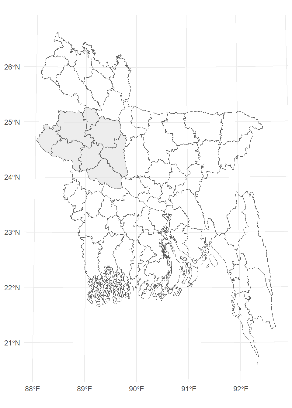

Geometry Union

Geometry union is a geospatial operation that involves combining multiple spatial features (points, lines, polygons) from different datasets into a single feature. The resulting feature represents the geometric union of the original features, effectively merging their boundaries and creating a new, larger feature that encompasses the area covered by the individual features. This operation is particularly useful for merging adjacent or overlapping features to create a more generalized representation.

First we will create eight shapefiles for each divisions using filter() function and write them to \Shapefiles\DB_DIVISIONS subfolder in a loo and then we will applyunction.

Code

unique_div <- unique(bd.div.st$ADM1_EN)
for( i in  unique_div){
  filter(bd.div.st, ADM1_EN == i) %>% 
  st_write(paste0(dataFolder,"\\Shapefiles\\DB_DIVISIONS\\", i, ".shp"), append= FALSE)
}

Deleting layer `Barisal' using driver `ESRI Shapefile'
Writing layer `Barisal' to data source 
  `G:\My Drive\Data\Bangladesh\\Shapefiles\DB_DIVISIONS\Barisal.shp' using driver `ESRI Shapefile'
Writing 1 features with 12 fields and geometry type Multi Polygon.
Deleting layer `Chittagong' using driver `ESRI Shapefile'
Writing layer `Chittagong' to data source 
  `G:\My Drive\Data\Bangladesh\\Shapefiles\DB_DIVISIONS\Chittagong.shp' using driver `ESRI Shapefile'
Writing 1 features with 12 fields and geometry type Multi Polygon.
Deleting layer `Dhaka' using driver `ESRI Shapefile'
Writing layer `Dhaka' to data source 
  `G:\My Drive\Data\Bangladesh\\Shapefiles\DB_DIVISIONS\Dhaka.shp' using driver `ESRI Shapefile'
Writing 1 features with 12 fields and geometry type Multi Polygon.
Deleting layer `Khulna' using driver `ESRI Shapefile'
Writing layer `Khulna' to data source 
  `G:\My Drive\Data\Bangladesh\\Shapefiles\DB_DIVISIONS\Khulna.shp' using driver `ESRI Shapefile'
Writing 1 features with 12 fields and geometry type Multi Polygon.
Deleting layer `Mymensingh' using driver `ESRI Shapefile'
Writing layer `Mymensingh' to data source 
  `G:\My Drive\Data\Bangladesh\\Shapefiles\DB_DIVISIONS\Mymensingh.shp' using driver `ESRI Shapefile'
Writing 1 features with 12 fields and geometry type Multi Polygon.
Deleting layer `Rajshahi' using driver `ESRI Shapefile'
Writing layer `Rajshahi' to data source 
  `G:\My Drive\Data\Bangladesh\\Shapefiles\DB_DIVISIONS\Rajshahi.shp' using driver `ESRI Shapefile'
Writing 1 features with 12 fields and geometry type Multi Polygon.
Deleting layer `Rangpur' using driver `ESRI Shapefile'
Writing layer `Rangpur' to data source 
  `G:\My Drive\Data\Bangladesh\\Shapefiles\DB_DIVISIONS\Rangpur.shp' using driver `ESRI Shapefile'
Writing 1 features with 12 fields and geometry type Multi Polygon.
Deleting layer `Sylhet' using driver `ESRI Shapefile'
Writing layer `Sylhet' to data source 
  `G:\My Drive\Data\Bangladesh\\Shapefiles\DB_DIVISIONS\Sylhet.shp' using driver `ESRI Shapefile'
Writing 1 features with 12 fields and geometry type Multi Polygon.

The union() function of raster package or spRbind() function of maptools package can be used to union two shape files. However, neither union() or spRbind() function can not join more than tow polygons at a time. So, you have to union polygons one by one. We have read the shape files as SPDF objects using raster::shapefile()

Code

# Load three shapefiles of three division
raj.sp<-raster::shapefile(paste0(dataFolder, "/Shapefiles/DB_DIVISIONS/Rajshahi.shp"))
rang.sp<-raster::shapefile(paste0(dataFolder, "/Shapefiles/DB_DIVISIONS/Rangpur.shp"))
khul.sp<-raster::shapefile(paste0(dataFolder, "/Shapefiles/DB_DIVISIONS/Khulna.shp"))

Code

# Union two division
division_02<-union(raj.sp, rang.sp)
division_03<-union(division_02, khul.sp)
## add another division
plot(division_03)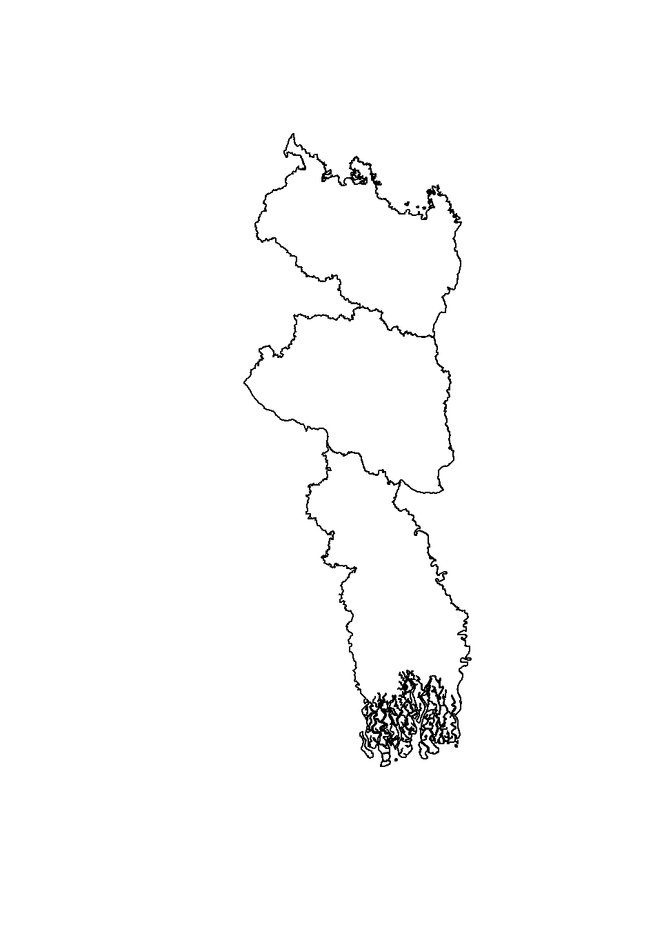

You can union hundreds of spatial polygons in a folder with similar geometry and attribute table using spRbind function of maptools package or union() function in a loop. First, you have to create a list these shape files using list.files() function, then use for loop to read all the files using readORG() function and then assign new feature IDs using spChFIDs() function of sp package, and finally apply spRbind() or union()to all files to union them. It is better to use spRbind function to union several polygons since it binds attribute data row wise.

Code

# create a list of file 
files <- list.files(path=paste0(dataFolder, ".//Shapefiles//DB_DIVISIONS"), pattern="*.shp$", recursive=TRUE, full.names=TRUE) # Create a list files
print(files)

[1] "G:\\My Drive\\Data\\Bangladesh\\.//Shapefiles//DB_DIVISIONS/Barisal.shp"   
[2] "G:\\My Drive\\Data\\Bangladesh\\.//Shapefiles//DB_DIVISIONS/Chittagong.shp"
[3] "G:\\My Drive\\Data\\Bangladesh\\.//Shapefiles//DB_DIVISIONS/Dhaka.shp"     
[4] "G:\\My Drive\\Data\\Bangladesh\\.//Shapefiles//DB_DIVISIONS/Khulna.shp"    
[5] "G:\\My Drive\\Data\\Bangladesh\\.//Shapefiles//DB_DIVISIONS/Mymensingh.shp"
[6] "G:\\My Drive\\Data\\Bangladesh\\.//Shapefiles//DB_DIVISIONS/Rajshahi.shp"  
[7] "G:\\My Drive\\Data\\Bangladesh\\.//Shapefiles//DB_DIVISIONS/Rangpur.shp"   
[8] "G:\\My Drive\\Data\\Bangladesh\\.//Shapefiles//DB_DIVISIONS/Sylhet.shp"

Code

uid<-1

# Get polygons from first file 
BD.DIV<- readOGR(files[1],gsub("^.*/(.*).shp$", "\\1", files[1]))

OGR data source with driver: ESRI Shapefile 
Source: "G:\My Drive\Data\Bangladesh\Shapefiles\DB_DIVISIONS\Barisal.shp", layer: "Barisal"
with 1 features
It has 12 fields

Code

n <- length(slot(BD.DIV, "polygons"))
BD.DIV <- spChFIDs(BD.DIV, as.character(uid:(uid+n-1)))
uid <- uid + n

# mapunit polygon: combin remaining  polygons with first polygoan
for (i in 2:length(files)) {
     temp.data <- readOGR(files[i], gsub("^.*/(.*).shp$", "\\1",files[i]))
     n <- length(slot(temp.data, "polygons"))
     temp.data <- spChFIDs(temp.data, as.character(uid:(uid+n-1)))
     uid <- uid + n
     #poly.data <- union(poly.data,temp.data)
     BD.DIV <- spRbind(BD.DIV,temp.data)
}

OGR data source with driver: ESRI Shapefile 
Source: "G:\My Drive\Data\Bangladesh\Shapefiles\DB_DIVISIONS\Chittagong.shp", layer: "Chittagong"
with 1 features
It has 12 fields
OGR data source with driver: ESRI Shapefile 
Source: "G:\My Drive\Data\Bangladesh\Shapefiles\DB_DIVISIONS\Dhaka.shp", layer: "Dhaka"
with 1 features
It has 12 fields
OGR data source with driver: ESRI Shapefile 
Source: "G:\My Drive\Data\Bangladesh\Shapefiles\DB_DIVISIONS\Khulna.shp", layer: "Khulna"
with 1 features
It has 12 fields
OGR data source with driver: ESRI Shapefile 
Source: "G:\My Drive\Data\Bangladesh\Shapefiles\DB_DIVISIONS\Mymensingh.shp", layer: "Mymensingh"
with 1 features
It has 12 fields
OGR data source with driver: ESRI Shapefile 
Source: "G:\My Drive\Data\Bangladesh\Shapefiles\DB_DIVISIONS\Rajshahi.shp", layer: "Rajshahi"
with 1 features
It has 12 fields
OGR data source with driver: ESRI Shapefile 
Source: "G:\My Drive\Data\Bangladesh\Shapefiles\DB_DIVISIONS\Rangpur.shp", layer: "Rangpur"
with 1 features
It has 12 fields
OGR data source with driver: ESRI Shapefile 
Source: "G:\My Drive\Data\Bangladesh\Shapefiles\DB_DIVISIONS\Sylhet.shp", layer: "Sylhet"
with 1 features
It has 12 fields

Code

BD.DIV@data

  Shape_Leng Shape_Area    ADM1_EN ADM1_PCODE ADM1_REF ADM1ALT1EN ADM1ALT2EN
1  25.424604  0.8893951    Barisal       BD10     <NA>       <NA>       <NA>
2  30.287321  2.7377958 Chittagong       BD20     <NA>       <NA>       <NA>
3  12.197758  1.8065059      Dhaka       BD30     <NA>       <NA>       <NA>
4  38.409385  1.8265749     Khulna       BD40     <NA>       <NA>       <NA>
5   8.166577  0.9418117 Mymensingh       BD45     <NA>       <NA>       <NA>
6   8.410221  1.6248559   Rajshahi       BD50     <NA>       <NA>       <NA>
7  15.369683  1.4656814    Rangpur       BD55     <NA>       <NA>       <NA>
8   9.800293  1.1039633     Sylhet       BD60     <NA>       <NA>       <NA>
     ADM0_EN ADM0_PCODE       date    validOn validTo
1 Bangladesh         BD 2015/01/01 2020/11/13    <NA>
2 Bangladesh         BD 2015/01/01 2020/11/13    <NA>
3 Bangladesh         BD 2015/01/01 2020/11/13    <NA>
4 Bangladesh         BD 2015/01/01 2020/11/13    <NA>
5 Bangladesh         BD 2015/01/01 2020/11/13    <NA>
6 Bangladesh         BD 2015/01/01 2020/11/13    <NA>
7 Bangladesh         BD 2015/01/01 2020/11/13    <NA>
8 Bangladesh         BD 2015/01/01 2020/11/13    <NA>

Code

plot(BD.DIV)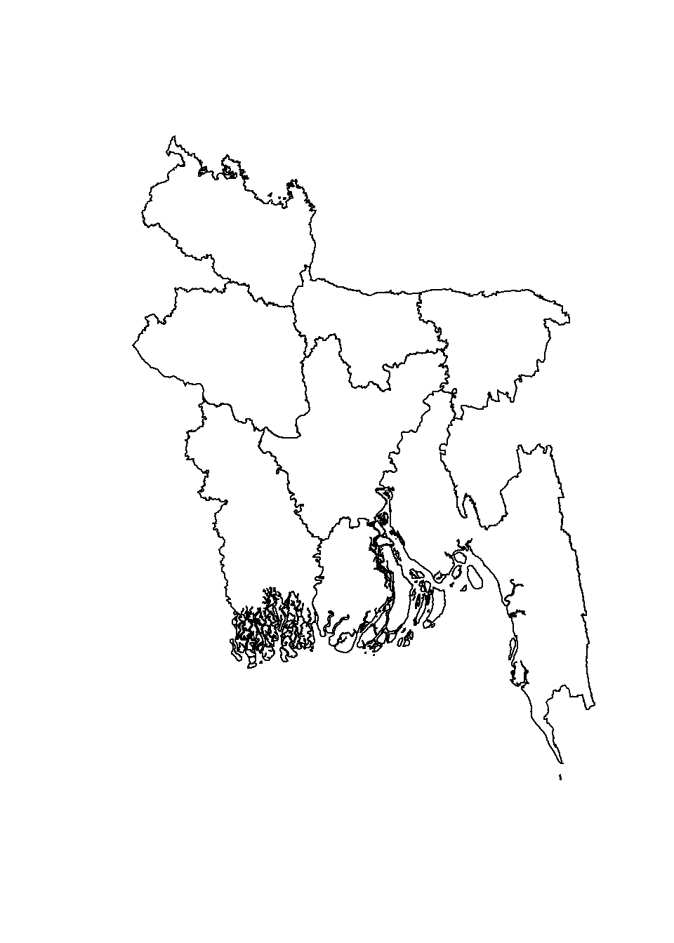

Geometry Dissolve

Dissolve aggregate features based on the attribute. It is an important tools that we may need to perform regularly in spatial data processing. This process effectively merges adjacent or overlapping polygons with the same attribute value into larger, simplified polygons. Dissolving is often used for generalization and simplification of spatial data, as well as for aggregating features based on shared attributes.

In R, you can perform spatial dissolve using the st_union() function from the sf package. We will dissolve all division boundary and create county boundary

Code

bd.div.st = sf::st_read("/vsicurl/https://github.com//zia207/r-colab/raw/main/Data/Bangladesh//Shapefiles/bd_division_BTM.shp")

Reading layer `bd_division_BTM' from data source 
  `/vsicurl/https://github.com//zia207/r-colab/raw/main/Data/Bangladesh//Shapefiles/bd_division_BTM.shp' 
  using driver `ESRI Shapefile'
Simple feature collection with 8 features and 12 fields
Geometry type: MULTIPOLYGON
Dimension:     XY
Bounding box:  xmin: 298487.8 ymin: 278578.1 xmax: 778101.8 ymax: 946939.2
Projected CRS: +proj=tmerc +lat_0=0 +lon_0=90 +k=0.9996 +x_0=500000 +y_0=-2000000 +datum=WGS84 +units=m +no_defs

Code

bd.bounadry<-st_union(bd.div.st)

Code

p1=ggplot() +
  geom_sf(data =bd.div.st, color = "grey", alpha = 0.7) +
  theme_minimal()
p2=ggplot() +
  geom_sf(data =bd.bounadry, color = "grey", alpha = 0.7) +
  theme_minimal()

Code

library(patchwork)
p1+p2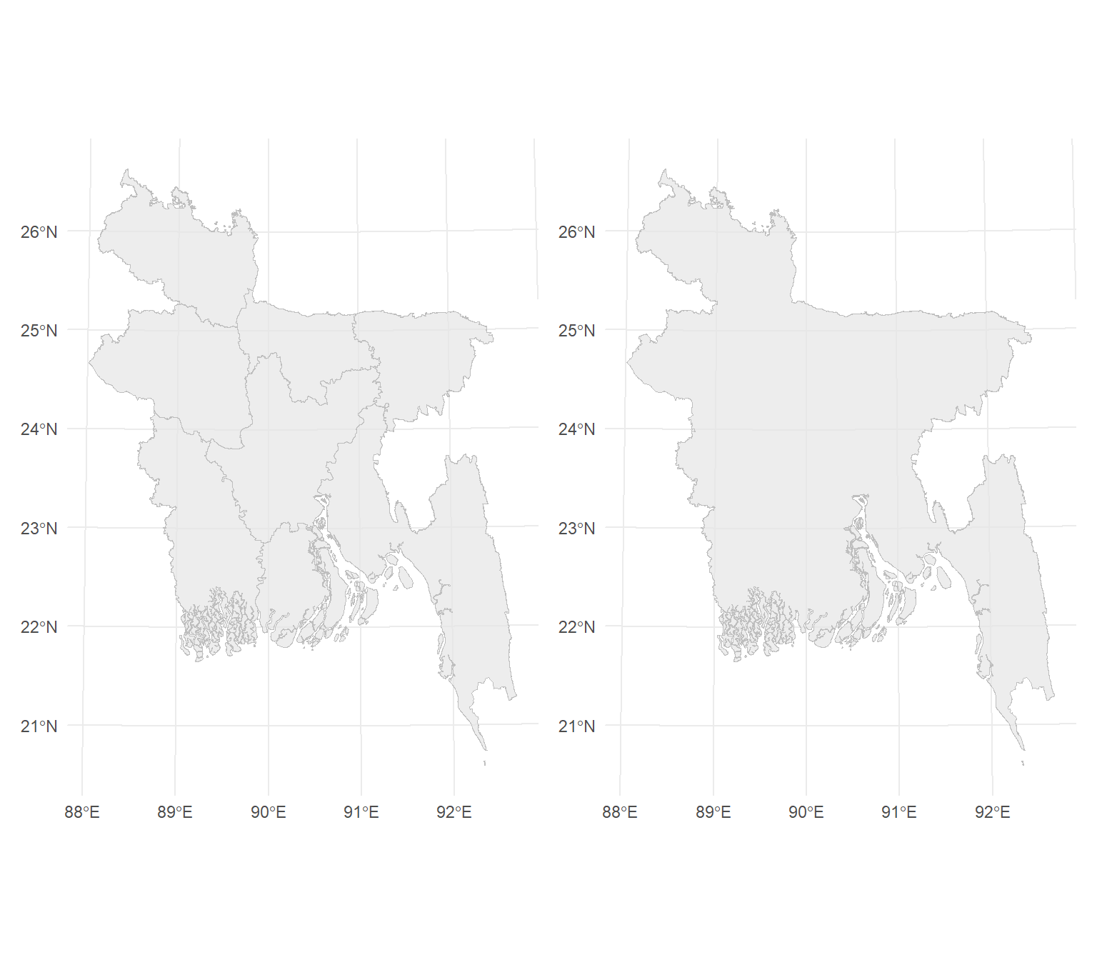

Geometry Simplification

Geometry simplification, also known as cartographic generalization, is the process of reducing the complexity of spatial geometries while preserving their essential shape and spatial relationships. This operation is often used to create simplified representations of geographic features for visualization, analysis, or storage, especially when dealing with large datasets or producing maps at different scales.

We will use a shape file entire Sundardban (both in India and Bangladesh) area to create a simplified geometry. In R, you can perform geometry simplification using the st_simplify() function with uses the **dTolerance* to control the level of generalization in map units.

Code

# define file from my github
sundarban.all = sf::st_read("/vsicurl/https://github.com//zia207/r-colab/raw/main/Data/Bangladesh//Shapefiles/sundarban_BTM.shp")

Reading layer `sundarban_BTM' from data source 
  `/vsicurl/https://github.com//zia207/r-colab/raw/main/Data/Bangladesh//Shapefiles/sundarban_BTM.shp' 
  using driver `ESRI Shapefile'
Simple feature collection with 2757 features and 10 fields
Geometry type: MULTIPOLYGON
Dimension:     XY
Bounding box:  xmin: 299728.6 ymin: 382775.2 xmax: 491618.5 ymax: 488820.4
Projected CRS: +proj=tmerc +lat_0=0 +lon_0=90 +k=0.9996 +x_0=500000 +y_0=-2000000 +datum=WGS84 +units=m +no_defs

Code

sundarban.simp = st_simplify(sundarban.all, dTolerance = 1000)  # 1000 m

The resulting simplified object is a copy of the original polygon but with fewer vertices

Code

p3=ggplot() +
  geom_sf(data =sundarban.all, color = "green", alpha = 0.7) +
  theme_minimal()+
  ggtitle("Orginal")
p4=ggplot() +
  geom_sf(data =sundarban.simp, color = "green", alpha = 0.7) +
  theme_minimal()+
  ggtitle("Simplified")

Code

library(patchwork)
p3+p4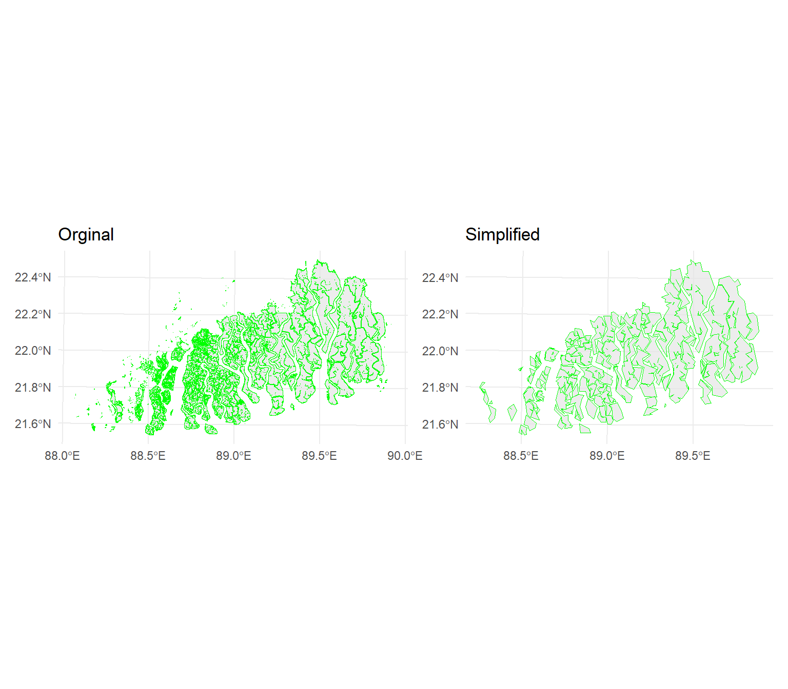

It also consuming less memory than the original object, as verified below:

Code

# Original
object.size(sundarban.all)

10104208 bytes

Code

# Simplified
object.size(sundarban.simp)

1485616 bytes

Geometric Intersections

Geometric intersections in spatial data involve determining the shared area or overlapping region between two or more spatial features (points, lines, polygons). This operation allows you to identify the locations where features intersect or overlap in space, which can be useful for various types of spatial analysis, such as identifying common boundaries, calculating overlap areas, or extracting features that fall within a specific region of interest.

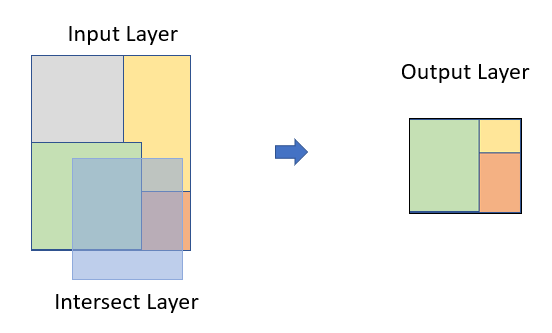
We will use a simplified ploygan of Sundardban (both in India and Bangladesh) to find out area that falls in Bangladesh. We perform a operation using st_intersection() function from the sf package

Code

# Apply intersect function  
sundarban.bd<- st_intersection(sundarban.simp, bd.bounadry)

Warning: attribute variables are assumed to be spatially constant throughout
all geometries

Code

p5=ggplot() +
  geom_sf(data =sundarban.simp, color = "green", alpha = 0.7) +
  #geom_sf(data =bd.bounadry, fill = "transparent") +
  theme_minimal()+
  ggtitle("Sundarban: India & Bangladesh")

p6=ggplot() +
  geom_sf(data =sundarban.bd, color = "green", alpha = 0.7) +
  #geom_sf(data =bd.bounadry, fill = "transparent") +
  theme_minimal()+
  ggtitle("Sundarban: Bangladesh")

Code

library(patchwork)
p5+p6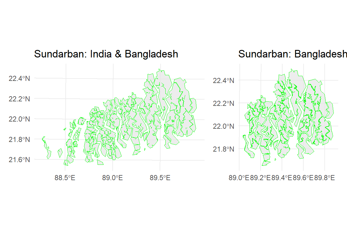

Geometry Erase

Erase() function in raster package erase parts of a SpatialPolygons or SpatialLines object with a another SpatialPolygons object. We will erase Rajshai division (raj.sp) from BD.DIV objects

Code

senven.DIV<-erase(BD.DIV, raj.sp)

Code

plot(senven.DIV)

Convex Hull

The convex hull is a geometric concept used in spatial analysis to define the smallest convex polygon that encloses a set of points or other geometric objects. In other words, it is the minimal convex shape that contains all the given points without any indentations or concave angles. The convex hull is often used to represent the outer boundary of a distribution of points or to simplify complex shapes for analysis and visualization.

Code

# define file from my github
point.st = sf::st_read("/vsicurl/https://github.com//zia207/r-colab/raw/main/Data/Bangladesh//Shapefiles/raj_soil_data_BTM.shp")

Reading layer `raj_soil_data_BTM' from data source 
  `/vsicurl/https://github.com//zia207/r-colab/raw/main/Data/Bangladesh//Shapefiles/raj_soil_data_BTM.shp' 
  using driver `ESRI Shapefile'
Simple feature collection with 5796 features and 34 fields
Geometry type: POINT
Dimension:     XY
Bounding box:  xmin: 303070.9 ymin: 635222.4 xmax: 481109.5 ymax: 794778.9
Projected CRS: +proj=tmerc +lat_0=0 +lon_0=90 +k=0.9996 +x_0=500000 +y_0=-2000000 +datum=WGS84 +units=m +no_defs

For creating a convex hull around a set of spatial points, you do following steps:

Convert sf object to spatial point dataframe (SPDF)

Code

SPDF <- sf:::as_Spatial(point.st$geom)

Get XY coordinates

Code

xy<-coordinates(SPDF)

Create convex hull

Code

CH.DF <- chull(xy)
# Closed polygon
coords <- xy[c(CH.DF, CH.DF[1]), ]

Plot them

Code

plot(xy, pch=19)
lines(coords, col="red")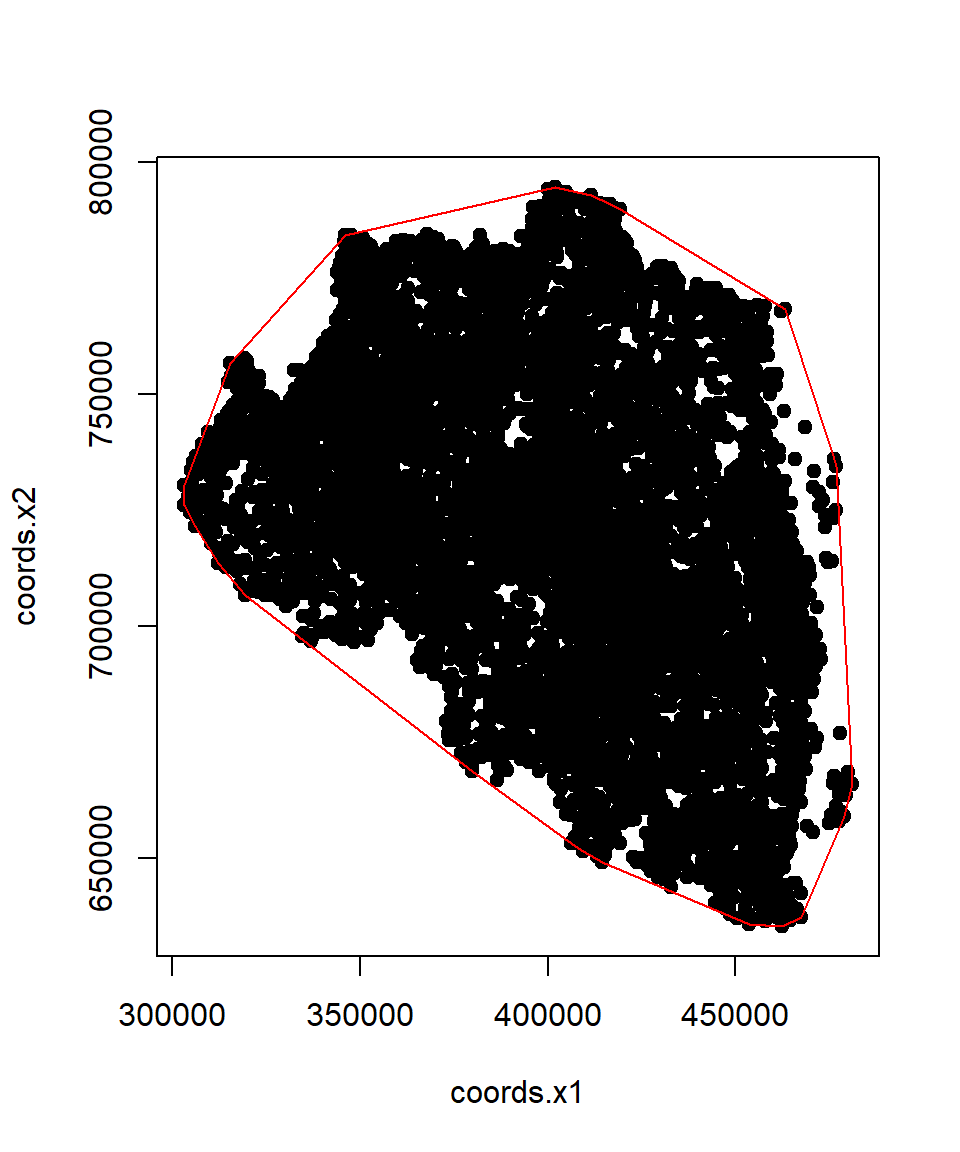

Buffer

Buffering is a common spatial analysis operation that involves creating a zone or area around spatial features such as points, lines, or polygons. This area is defined by a specified distance or buffer distance from the original feature. Buffering is useful for tasks like proximity analysis, identifying features within a certain distance of other features, or delineating areas of influence.

Buffering of Polylines

Code

raj.div.road<-sf::st_read("/vsicurl/https://github.com//zia207/r-colab/raw/main/Data/Bangladesh//Shapefiles/raj_road_BTM.shp")

Reading layer `raj_road_BTM' from data source 
  `/vsicurl/https://github.com//zia207/r-colab/raw/main/Data/Bangladesh//Shapefiles/raj_road_BTM.shp' 
  using driver `ESRI Shapefile'
Simple feature collection with 1596 features and 7 fields
Geometry type: MULTILINESTRING
Dimension:     XY
Bounding box:  xmin: 307989 ymin: 635678.6 xmax: 480663.6 ymax: 795730.6
Projected CRS: +proj=tmerc +lat_0=0 +lon_0=90 +k=0.9996 +x_0=500000 +y_0=-2000000 +datum=WGS84 +units=m +no_defs

Code

plot(raj.div.road$geometry)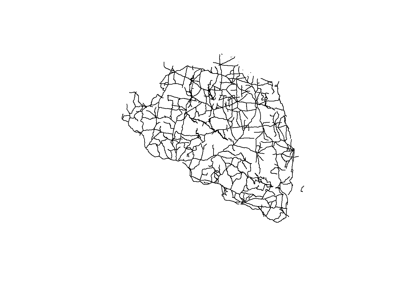

First we will create polylines for the national highway for the Rajshahi Division

Code

raj.highway <-raj.div.road %>%
  filter(ROADCLASS == "National highway")

you can perform buffering using the st_buffer() function from the sf package. Here’s how you can use it for 2 Km buffer:

Code

road_buff_2km = st_buffer(raj.highway, dist = 2000)

Code

plot(road_buff_2km$geometry, main="2000 m Buffer")
plot(raj.highway ,add=TRUE, col="red")

Warning in plot.sf(raj.highway, add = TRUE, col = "red"): ignoring all but the
first attribute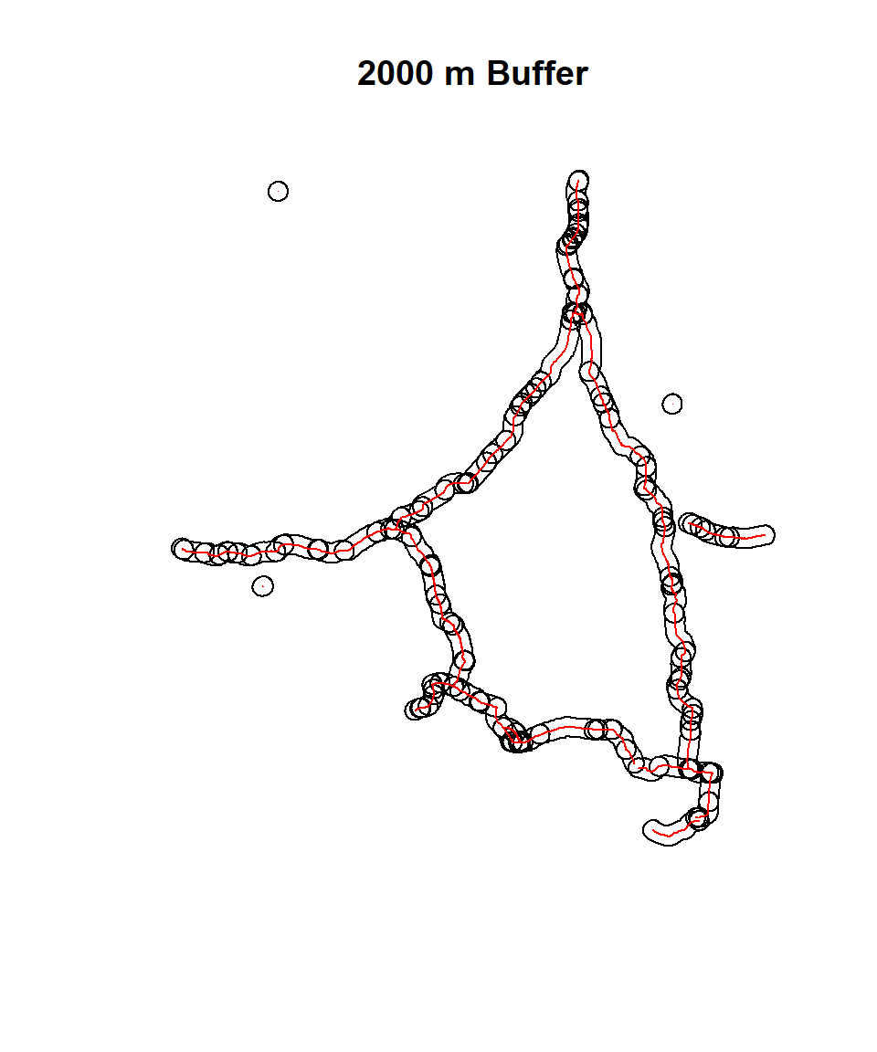

Buffering of Point data

Code

# define file from my github
raj.soil = sf::st_read("/vsicurl/https://github.com//zia207/r-colab/raw/main/Data/Bangladesh//Shapefiles/raj_soil_data_BTM.shp")

Reading layer `raj_soil_data_BTM' from data source 
  `/vsicurl/https://github.com//zia207/r-colab/raw/main/Data/Bangladesh//Shapefiles/raj_soil_data_BTM.shp' 
  using driver `ESRI Shapefile'
Simple feature collection with 5796 features and 34 fields
Geometry type: POINT
Dimension:     XY
Bounding box:  xmin: 303070.9 ymin: 635222.4 xmax: 481109.5 ymax: 794778.9
Projected CRS: +proj=tmerc +lat_0=0 +lon_0=90 +k=0.9996 +x_0=500000 +y_0=-2000000 +datum=WGS84 +units=m +no_defs

First we will create soil point data frame for Bogra district, then we will apply st_buffer() function

Code

bogra.soil <-raj.soil %>%
  filter(DIST_NAME == "BOGRA")

Code

point.buffer <-st_buffer(bogra.soil,  dist = 1000) # 1 km buffer

Code

ggplot() +
  geom_sf(data =point.buffer, color = "green", alpha = 0.7) +
  geom_sf(data =bogra.soil, fill = "transparent") +
  theme_minimal()+
  ggtitle("Point buffer: 1 Km")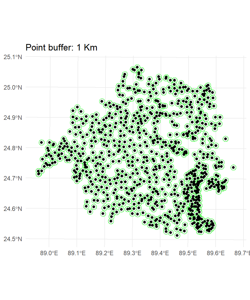

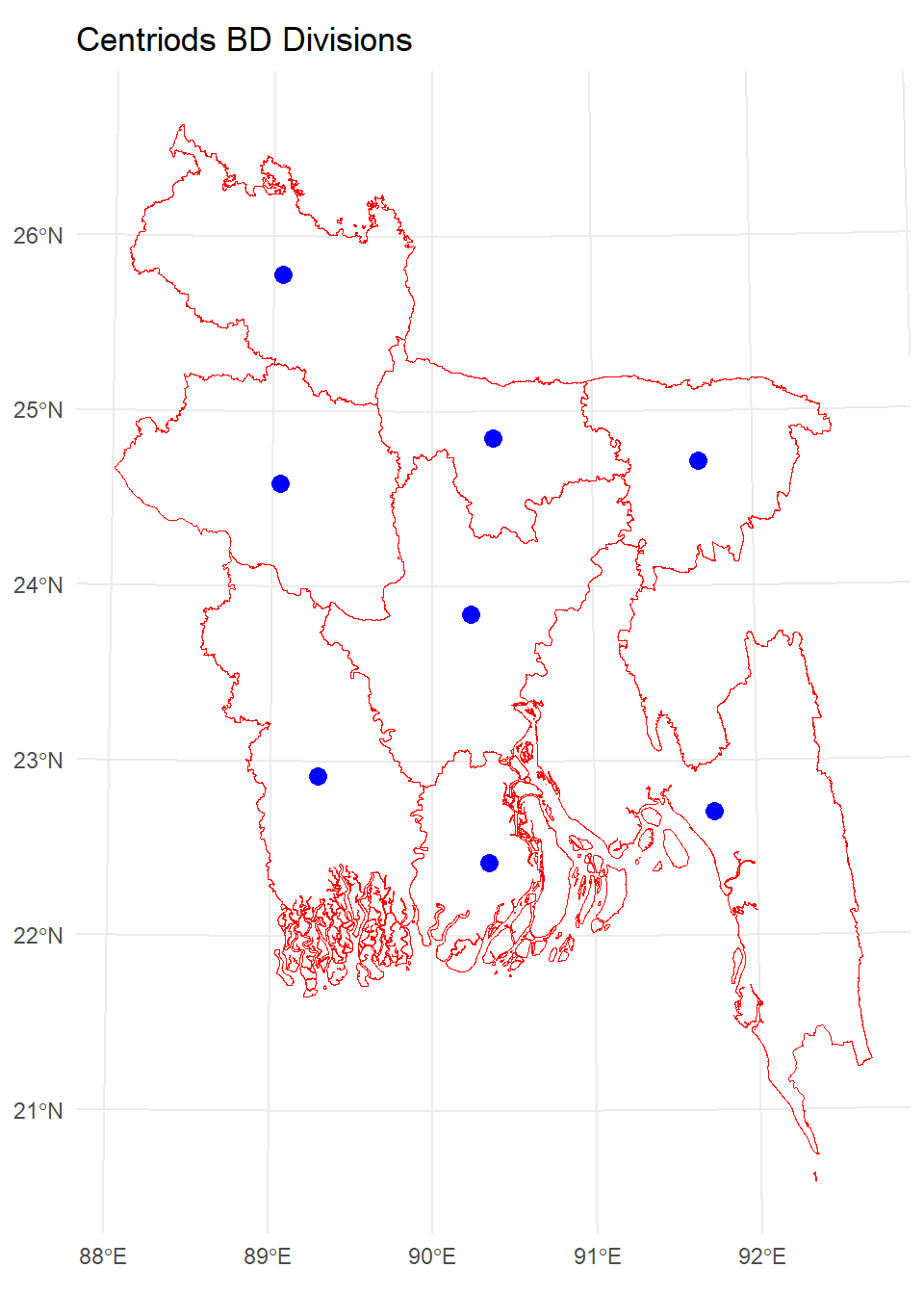
Centroids

A centroid is a point that represents the geometric center or average location of a spatial feature, such as a polygon. It is calculated based on the shape and distribution of the feature’s vertices. Centroids are often used for labeling features, performing spatial analysis, or representing the “center of mass” of an object.

In R, you can calculate centroids using the st_centroid() function from the sf package. Here’s how you can use it:

Code

bd.div.st = sf::st_read("/vsicurl/https://github.com//zia207/r-colab/raw/main/Data/Bangladesh//Shapefiles/bd_division_BTM.shp")

Reading layer `bd_division_BTM' from data source 
  `/vsicurl/https://github.com//zia207/r-colab/raw/main/Data/Bangladesh//Shapefiles/bd_division_BTM.shp' 
  using driver `ESRI Shapefile'
Simple feature collection with 8 features and 12 fields
Geometry type: MULTIPOLYGON
Dimension:     XY
Bounding box:  xmin: 298487.8 ymin: 278578.1 xmax: 778101.8 ymax: 946939.2
Projected CRS: +proj=tmerc +lat_0=0 +lon_0=90 +k=0.9996 +x_0=500000 +y_0=-2000000 +datum=WGS84 +units=m +no_defs

Code

div.centroids <- st_centroid(bd.div.st)

Warning: st_centroid assumes attributes are constant over geometries

Code

ggplot() +
  geom_sf(data = div.centroids, color = "blue", size = 3) +
  geom_sf(data = bd.div.st, fill = "transparent", color = "red") +
  theme_minimal()+
  ggtitle("Centriods BD Divisions")

Geometric Operations on Vector Data

Load Packages

Data

Spatial Clipping

Geometry Union

Geometry Dissolve

Geometry Simplification

Geometric Intersections

Geometry Erase

Convex Hull

Buffer

Buffering of Polylines

Buffering of Point data

Centroids

Further Reading