Artificial Neural Networks (ANNs)
Artificial Neural Networks (ANNs) are a class of machine learning models that are inspired by the structure and function of biological neural networks, such as the human brain. ANNs consist of interconnected nodes, called artificial neurons or nodes, which process and transmit information using a set of weighted connections.
The hidden layers in a deep neural network enable the model to learn multiple levels of abstraction, where each layer learns and extracts higher-level representations of the input data. The input layer receives the raw input data, and the output layer produces the final prediction or classification. The intermediate layers, known as hidden layers, perform computations and transformations on the input data to extract relevant features.
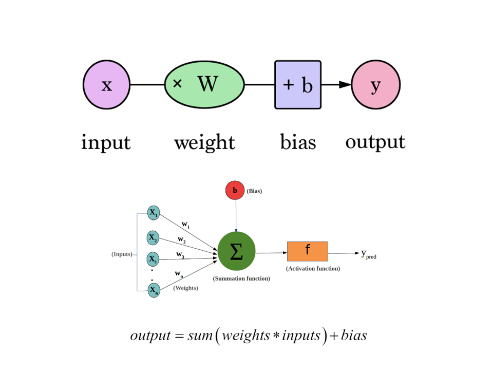
The basic idea behind ANNs is to simulate the behavior of biological neurons in a computational model. Each artificial neuron takes in one or more inputs, applies a weighted sum to the inputs, and passes the result through an activation function to produce an output. The activation function introduces non-linearity and enables the network to learn complex patterns in the data.
ANNs are organized into layers of neurons. The input layer receives the input data, and the output layer produces the final prediction or classification. In between, there can be one or more hidden layers, which perform the bulk of the computation in the network. Each neuron in a hidden layer receives input from the neurons in the previous layer and produces an output based on its weights and biases.
During training, the weights and biases of the neurons in the network are adjusted using an optimization algorithm, such as back-propagation, to minimize the difference between the predicted and actual outputs. The training process involves feeding the network with labeled training data, computing the error or loss, and updating the weights and biases iteratively until the network learns to make accurate predictions.
A perceptron is the simplest form of an ANN that consists of a single artificial neuron or node. It is a binary classification algorithm that can be used to learn a linear decision boundary for separating two classes of data.
A Deep Neural Network (DNN) is a type of artificial neural network (ANN) that consists of multiple layers of interconnected artificial neurons or nodes. It is called “deep” because it has a significant number of hidden layers, allowing it to learn complex patterns and hierarchies of features from input data.
ANNs have gained popularity due to their ability to learn from complex and high-dimensional data, as well as their capability to generalize and make predictions on new, unseen data. They have been successfully applied in various domains, including computer vision, natural language processing, speech recognition, and many other areas of machine learning and artificial intelligence.
Architecture of a Neural Network
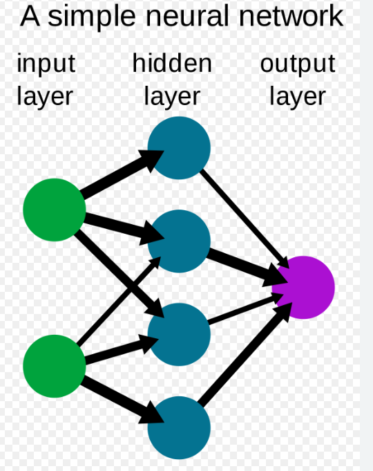
A simple neural network architecture typically consists of an input layer, one or more hidden layers, and an output layer.
The input layer receives the input data, which could be anything from an image to a set of numerical features. Each neuron in the input layer represents a single feature of the input data.
The hidden layer(s) perform the bulk of the computation in the network. Each neuron in a hidden layer receives input from the neurons in the previous layer and produces an output based on its weights and biases. The number of neurons in the hidden layer(s) can vary depending on the complexity of the problem being solved.
The output layer produces the final output of the network. It typically contains one neuron for each possible output class or value. The output of each neuron represents the probability of the input data belonging to that class or having that value.
During training, the weights and biases of the neurons in the network are adjusted using a learning algorithm such as backpropagation, to minimize the difference between the predicted and actual outputs.
Steps in Neural Network
The steps involved in training and using a neural network can be summarized as follows:
Data Preparation: Collect and preprocess the training data. This may involve tasks such as cleaning the data, handling missing values, normalizing or scaling the features, and splitting the data into training and validation sets.
Network Architecture Design: Determine the architecture of the neural network, including the number of layers, the number of neurons in each layer, and the choice of activation functions for each layer. This step depends on the specific problem you are trying to solve. The input data is fed into the input layer of the neural network. Each node in the input layer represents a feature or attribute of the data. Then, the input data is passed through one or more hidden layers. Each hidden layer consists of multiple neurons, and the activations from the previous layer serve as inputs to the neurons in the current layer.
Initialize Parameters: Initialize the weights and biases of the neural network with random values. Proper initialization is important to prevent the network from getting stuck in local optima.
Forward Propagation: Perform forward propagation by feeding the training data through the network. This step produces the predicted output of the network. In each neuron of the hidden layers, the inputs are multiplied by the corresponding weights. These weighted inputs are summed together to compute a weighted sum for each neuron. After the weighted sum is calculated, an activation function is applied to introduce non-linearity and determine the output of each neuron. Common activation functions include sigmoid, ReLU, tanh, and softmax, depending on the layer and the problem being solved.
Compute Loss: Calculate the loss or error between the predicted output and the actual output. The choice of loss function depends on the type of problem, such as mean squared error for regression or cross-entropy loss for classification.
Backpropagation: Perform backpropagation to compute the gradients of the loss function with respect to the weights and biases of the network. This step involves calculating the error contributions of each neuron and propagating them backward through the layers.
Update Parameters: Update the weights and biases of the network using an optimization algorithm such as gradient descent. The learning rate determines the step size of the parameter updates.
Repeat Steps 4-7: Repeat steps 4 to 7 for a specified number of epochs or until the desired level of convergence is reached. Each iteration of forward propagation, loss computation, backpropagation, and parameter update improves the network’s performance.
Model Evaluation: Evaluate the trained model on a separate validation set or test set to assess its performance. Metrics such as accuracy, precision, recall, and F1 score can be used to evaluate classification models, while mean squared error or R-squared can be used for regression models.
Prediction: Once the model is trained and evaluated, it can be used to make predictions on new, unseen data by performing forward propagation on the input.
It’s important to note that these steps are a general guideline, and the specific implementation may vary depending on the neural network framework or library being used.
Some Important Terminologies
Weights and Biases
In machine learning and neural networks, weights and biases are the learnable parameters that are used to represent the relationships between the input features and the output predictions.
Weights are the parameters that are multiplied by the input values to produce the output of a neuron in a neural network. Each connection between two neurons in a network has a weight associated with it, which determines the strength of the connection. During the training process, the weights are adjusted by the optimization algorithm to minimize the error or loss function.
Biases, on the other hand, are added to the weighted sum of inputs to a neuron to produce the output. They represent the inherent bias or offset in the data, and help the network to generalize better to new, unseen data. Like weights, biases are also adjusted during the training process to minimize the error or loss function.
Together, the weights and biases of a neural network form the model parameters that are learned during the training process. The optimization algorithm works by adjusting these parameters to minimize the error or loss function, and in doing so, improve the accuracy of the model’s predictions. The process of learning the optimal weights and biases for a given neural network is often referred to as model training.
Forward Propoagation
Forward propagation is the process of computing the outputs of a neural network given an input. It involves passing the input data through the network’s layers, performing computations, and producing the final output or prediction.
Activation Functions
In neural networks, activation functions are used to introduce non-linearity to the output of a neuron or a layer. They transform the input signal to the output signal of a neuron or a layer, which is then passed to the next layer or output.
Activation functions are essential in neural networks because they enable the network to learn complex non-linear relationships between the input and output data. Without activation functions, neural networks would simply be linear transformations, which are not capable of modeling complex patterns in the data.
There are several types of activation functions commonly used in neural networks, including:
Sigmoid: The sigmoid function maps the input values to a range between 0 and 1, making it useful for binary classification problems.
ReLU (Rectified Linear Unit): The ReLU function sets the output to zero for any negative input values, and linearly increases the output for positive input values. ReLU is commonly used in deep learning because it is computationally efficient and can avoid the vanishing gradient problem.
Tanh (Hyperbolic tangent): The Tanh function maps the input values to a range between -1 and 1, making it useful for classification problems.
Softmax: The softmax function is used in the output layer of a classification network to produce a probability distribution over the output classes.
Leaky ReLU: Leaky ReLU is similar to ReLU, but instead of setting the output to zero for negative input values, it introduces a small negative slope, allowing for non-zero output for negative input values.
The choice of activation function depends on the specific problem being solved and the architecture of the neural network. Different activation functions can have different computational properties, such as differentiability and monotonicity, which can affect the optimization process and the accuracy of the model’s predictions.
Back-propagation
Backpropagation is a supervised learning algorithm used for training Artificial Neural Networks (ANNs). It is a method for computing the gradient of the loss function with respect to the weights and biases of the neurons in the network, and using this gradient to update the weights and biases in order to minimize the error in the network’s predictions.
The backpropagation algorithm works by propagating the error backwards through the network, from the output layer to the input layer. It computes the error at each layer by taking the derivative of the loss function with respect to the output of that layer, and then propagating this error backwards to the previous layers.
The algorithm can be summarized in the following steps:
Forward propagation: The input data is fed into the network, and the output of each neuron is computed using the current weights and biases.
Compute the error: The error between the predicted output and the actual output is computed using a loss function.
Backward propagation: The error is then propagated backwards through the network, starting from the output layer to the input layer. At each layer, the error is computed by taking the derivative of the loss function with respect to the output of that layer.
Update weights and biases: The gradient of the loss function with respect to the weights and biases of each neuron is computed using the chain rule, and the weights and biases are then updated in the direction that reduces the error.
Repeat steps 1 to 4: Steps 1 to 4 are repeated multiple times, or epochs, until the error is minimized or a stopping criterion is met.
Backpropagation is a powerful algorithm that has enabled the training of deep neural networks with many layers. However, it can suffer from problems such as vanishing gradients and overfitting, which require additional techniques such as regularization and adaptive learning rate methods to overcome.
Loss function
In machine learning, a loss function, also known as a cost function or an objective function, is a function that measures the difference between the predicted output and the actual output for a given input. It is used to quantify the error or the deviation between the predicted output of a model and the actual output.
The choice of a suitable loss function depends on the type of problem being solved. For example, in regression problems, where the goal is to predict a continuous output, a common loss function is the mean squared error (MSE), which measures the average squared difference between the predicted output and the actual output. In classification problems, where the goal is to predict a discrete output, a common loss function is the cross-entropy loss, which measures the difference between the predicted probabilities and the actual probabilities of each class.
The loss function plays a critical role in training machine learning models, as it provides the basis for the optimization algorithm to adjust the model parameters such as the weights and biases of the neural network, so as to minimize the error. The process of minimizing the loss function is typically achieved through a process called gradient descent, which involves computing the gradient of the loss function with respect to the model parameters, and updating them in the direction that reduces the loss.
In summary, the loss function is a fundamental component of any machine learning model, and its choice and design are critical to the success of the model in solving a given problem.
Gradient Descent
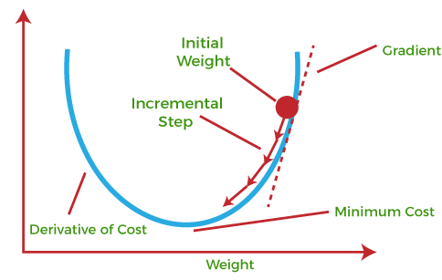
Gradient descent is an optimization algorithm commonly used in machine learning to minimize a cost or loss function. It is an iterative algorithm that adjusts the parameters of a model in the direction of steepest descent of the cost function.
The main idea behind gradient descent is to update the model parameters by taking steps proportional to the negative gradient of the cost function with respect to the parameters. The negative gradient represents the direction of the steepest descent, and by moving in that direction, the algorithm aims to find the minimum of the cost function.
Here are the key steps involved in gradient descent:
Initialize parameters: The algorithm starts by initializing the model parameters, such as the weights and biases, with some initial values.
Compute the gradient: The gradient of the cost function with respect to the parameters is computed. The gradient represents the direction and magnitude of the steepest ascent of the cost function.
Update parameters: The parameters are updated by taking a step in the opposite direction of the gradient. The size of the step is determined by the learning rate, which is a hyperparameter that controls the step size. The learning rate determines how quickly or slowly the algorithm converges to the minimum.
Repeat steps 2 and 3: Steps 2 and 3 are repeated iteratively until a stopping criterion is met. This could be a fixed number of iterations, reaching a certain level of convergence, or other termination conditions.
There are different variants of gradient descent, such as batch gradient descent, stochastic gradient descent, and mini-batch gradient descent. These variants differ in the amount of data used to compute the gradient and update the parameters at each iteration.
Gradient descent is a fundamental optimization algorithm in machine learning, and it is widely used for training various models, including neural networks. It allows models to learn from data by iteratively adjusting the parameters to minimize the cost function, resulting in better predictions and improved model performance.
Dropout layer
A dropout layer is a regularization technique commonly used in deep neural networks to prevent overfitting and improve generalization. It randomly sets a fraction of the input units (neurons) to zero at each training iteration, effectively “dropping out” those units temporarily. The dropout layer is typically inserted between the hidden layers of a neural network. During training, for each training example, the dropout layer randomly masks (sets to zero) a specified fraction of the input units. The fraction, known as the dropout rate, is a hyperparameter that determines the proportion of units to be dropped out. The remaining units are then rescaled by a factor of 1/(1 - dropout rate) to compensate for the missing units. This scaling ensures that the expected sum of the units remains constant, maintaining the average magnitude of the activations.
Learning Rate
The learning rate is a hyperparameter that controls the step size at which the parameters (weights and biases) of a neural network are updated during the training process. It determines how quickly or slowly the model learns from the gradients computed during backpropagation.
Finding an appropriate learning rate is crucial for effective training. Here are some considerations:
Too high learning rate: If the learning rate is too high, the optimization process may become unstable, and the loss function may not converge. The model may exhibit large oscillations or even diverge. In such cases, reducing the learning rate can help stabilize the training process.
Too low learning rate: If the learning rate is too low, the optimization process may become slow, and the model may take a long time to converge. It may get stuck in suboptimal solutions or plateaus. In such cases, increasing the learning rate can speed up the convergence.
Learning rate decay: It is common to decay the learning rate over time as training progresses. Starting with a higher learning rate and gradually reducing it can help the model initially explore the parameter space broadly and then fine-tune the parameters for better convergence.
Learning rate scheduling: Instead of a fixed learning rate, it is also possible to use learning rate scheduling techniques, where the learning rate is adjusted based on certain criteria or events during training. For example, learning rate can be reduced if the validation loss stops improving or if the training loss reaches a certain threshold.
Choosing the right learning rate requires experimentation and tuning. It is often recommended to start with a relatively small learning rate and gradually increase or decrease it based on the observed performance during training. Techniques like grid search or automated hyperparameter optimization can also be used to find an optimal learning rate.
Different optimization algorithms, such as Adam, RMSProp, or SGD (Stochastic Gradient Descent), may have their own ways of handling the learning rate. Therefore, it’s important to consider the interaction between the learning rate and the specific optimization algorithm being used.
Overall, the learning rate plays a critical role in training neural networks, and finding the right balance is essential for achieving efficient convergence and good generalization performanc.
Adaptive Learning rate
Adaptive learning rate refers to the technique of dynamically adjusting the learning rate during the training process of a neural network. The learning rate determines the step size at which the model’s parameters (weights and biases) are updated during gradient descent or other optimization algorithms.
The purpose of adaptive learning rate methods is to improve the efficiency and effectiveness of the training process by automatically adjusting the learning rate based on the characteristics of the optimization problem. This is particularly useful when dealing with complex and high-dimensional datasets where the optimal learning rate may vary across different stages or dimensions of the optimization process.
There are several popular adaptive learning rate algorithms, including:
Adagrad (Adaptive Gradient): Adagrad adapts the learning rate for each parameter based on the historical squared gradients. It accumulates the squared gradients over time and performs smaller updates for parameters with large gradients and larger updates for parameters with smaller gradients.
RMSProp (Root Mean Square Propagation): RMSProp modifies Adagrad by using an exponentially decaying average of squared gradients. It maintains a running average of the squared gradients and adjusts the learning rate accordingly. This helps to normalize the learning rates and overcome the diminishing learning rate problem in Adagrad.
Adam (Adaptive Moment Estimation): Adam combines the ideas of both Adagrad and RMSProp. It maintains running averages of both the gradients and the squared gradients, and it incorporates bias correction. Adam adapts the learning rate based on both the first moment (mean) and the second moment (variance) of the gradients.
These adaptive learning rate algorithms allow the learning rate to be adjusted automatically based on the current state of the optimization process. By adapting the learning rate, these methods can help overcome challenges such as slow convergence, vanishing or exploding gradients, and finding a suitable learning rate for different parameters or stages of training.
Applying adaptive learning rate techniques can often lead to faster convergence, better exploration of the optimization landscape, and improved overall performance of the neural network. However, the choice of the adaptive learning rate algorithm and its hyperparameters should be carefully considered and tuned based on the specific problem and dataset to achieve the best results.
Further Reading
YouTube Video
Neural Networks Pt. 1: Inside the Black Box
Source: StatQuest with Josh StarmeOverview | Neural Networks
Source: First Principles of Computer Vision
Perceptron | Neural Networks
Source: First Principles of Computer Vision
Activation Function | Neural Networks
Source: First Principles of Computer Vision
Neural Networks Pt. 2: Backpropagation Main Ideas
Source: StatQuest with Josh Starme
Gradient Descent | Neural Networks