Map Projection and Coordinate Reference Systems in R
Coordinate Reference Systems
Coordinate Reference Systems (CRS) are used in cartography, geography, and GIS (Geographic Information Systems) to define the positions of points, lines, and areas on the Earth’s surface. A CRS provides a framework for translating geographic locations, which are expressed as latitude and longitude or other coordinate values, into a specific location on a map or a two-dimensional plane.
There are two main types of Coordinate Reference Systems:
Geographic Coordinate Systems (GCS): Geographic Coordinate Systems use latitude and longitude to define locations on the Earth’s surface. Latitude measures the north-south position, while longitude measures the east-west position. The coordinates are expressed in degrees, minutes, and seconds or decimal degrees. Common GCS examples include WGS 84 (World Geodetic System 1984) and NAD83 (North American Datum 1983).
Projected Coordinate Systems (PCS): Projected Coordinate Systems use Cartesian coordinates (X, Y) to represent locations on a flat, two-dimensional map. The projection converts the three-dimensional geographic coordinates (latitude, longitude, and often elevation) into these two-dimensional coordinates. Different map projections, such as Mercator, Robinson, or UTM (Universal Transverse Mercator), create projected coordinate systems.
Source: ESRI
The equidistant lines that run east and west each have a constant latitude value called parallels. The equator is the largest circle and divides the earth in half. It is equal in distance from each of the poles, and the value of this latitude line is zero. Locations north of the equator has positive latitudes that range from 0 to +90 degrees, while locations south of the equator have negative latitudes that range from 0 to -90 degrees.
The lines that run through north and south each have a constant longitude value and form circles of the same size around the earth known as meridians. The prime meridian is the line of longitude that defines the origin (zero degrees) for longitude coordinates. One of the most commonly used prime meridian locations is the line that passes through Greenwich, England. Locations east of the prime meridian up to its antipodal meridian (the continuation of the prime meridian on the other side of the globe) have positive longitudes ranging from 0 to +180 degrees. Locations west of the prime meridian has negative longitudes ranging from 0 to -180 degrees.
The latitude and longitude lines cover the globe to form a grid that know as a graticule. The point of origin of the graticule is (0,0), where the equator and the prime meridian intersect. The equator is the only place on the graticule where the linear distance corresponding to one degree latitude is approximately equal the distance corresponding to one degree longitude. Because the longitude lines converge at the poles, the distance between two meridians is different at every parallel.
To maintain accuracy in GIS and cartographic applications, it’s essential to use the appropriate coordinate reference system and datum for the specific region or project. Choosing the wrong CRS can lead to distortions and inaccuracies when transforming between geographic locations and map coordinates.
CRS is a fundamental aspect of spatial data management, as they allow for the integration of different data sources, analysis, and visualization of geographic information consistently and meaningfully. Understanding CRS is crucial for cartographers, GIS analysts, and anyone working with geographic data to ensure accurate spatial representation and analysis.
Map Projection
Map projection is a method used to represent the three-dimensional surface of the Earth on a two-dimensional map. Since the Earth is a spherical object, it is challenging to depict its curved surface accurately on a flat surface. This problem arises because representing the entire curved surface of the Earth on a flat map results in distortions in shape, size, distance, or direction.
Various map projections are available, each designed to address different needs and minimize certain types of distortion. Here are some common types of map projections:
Mercator Projection: Developed by Gerardus Mercator in the 16th century, this projection preserves straight lines, making it useful for marine navigation. However, it distorts the sizes of landmasses, with areas near the poles appearing significantly more significant than they are.
Robinson Projection: This compromise projection attempts to balance size, shape, and distance distortions across the entire map. It’s commonly used for world maps.
Conic Projection: This projection involves projecting the Earth’s surface onto a cone and then unrolling the cone to form a flat map. It preserves shapes and distances well within the cone area but can have significant distortions as one moves away from that central area.
Cylindrical Projection: This projection wraps the Earth’s surface around a cylinder. Examples include the Mercator projection mentioned earlier and the Miller projection, which preserves relative size but distorts shapes.
Azimuthal Projection: These projections project the Earth’s surface onto a plane from a specific point on the Earth’s surface. They preserve directionality but can have considerable distortions in other aspects.
Goode’s Homolosine Projection: This projection combines the sinusoidal and Mollweide projection to reduce landmass size distortion, although it sacrifices shape accuracy.
The choice of map projection depends on the intended use of the map, the area being represented, and the extent to which certain distortions are acceptable. No single projection can perfectly represent the entire Earth without any distortions, and mapmakers must make trade-offs based on their specific needs.
It’s important to understand that map projections are just one aspect of cartography, and producing accurate and valuable maps often involves other techniques, such as generalization, symbolization, and labeling.
The World Geodetic System 1984 (WGS 84) is a global geodetic reference system developed and maintained by the United States Department of Defense (DoD). It is widely used as the standard coordinate reference system for the Earth’s surface in various applications, including mapping, navigation, surveying, and GPS (Global Positioning System).
WGS 84 is an Earth-centered, Earth-fixed coordinate system known as a geocentric coordinate system. It defines a three-dimensional model of the Earth, where the center of the Earth serves as the origin, and the X, Y, and Z axes are oriented with respect to the Earth’s rotation and equator.
The key features of WGS 84 include:
Ellipsoid: WGS 84 uses the WGS 84 ellipsoid, a mathematically defined surface approximating the shape of the Earth. It is an oblate spheroid, slightly flattened at the poles and bulging at the equator.
Datum: WGS 84 defines a specific datum, which includes the ellipsoid’s size, shape, and orientation in relation to the Earth’s center. The datum is a reference frame for measuring positions on the Earth’s surface.
Coordinate Units: WGS 84 uses degrees of latitude and longitude to express geographic positions. Latitude measures the north-south position, and longitude measures the east-west position.
GPS Reference Frame: WGS 84 is the coordinate system used by the Global Positioning System (GPS). GPS receivers use WGS 84 to accurately determine the user’s position on the Earth’s surface.
Constantly Updated: The WGS 84 reference frame is continuously refined and updated to account for crustal movements, which can affect the Earth’s shape and position. As such, newer versions of WGS 84 have been released, with slight adjustments to improve accuracy.
The adoption of WGS 84 as a global standard has been instrumental in enabling accurate navigation, mapping, and geospatial data exchange across the world. It ensures consistency and interoperability among different mapping and navigation systems, making it possible to integrate data from various sources into a coherent spatial framework.
The Universal Transverse Mercator (UTM) is a widely used map projection and coordinate reference system that divides the Earth’s surface into a series of zones, each with its own unique coordinate system. It is designed to minimize distortion within each zone, making it suitable for accurate mapping and navigation in relatively small areas.
The UTM projection is a type of cylindrical projection that projects the Earth’s surface onto a cylinder. The cylinder is then unwrapped to create a flat map. The key features of the UTM system include:
Zone System: The Earth is divided into 60 longitudinal zones, each spanning 6 degrees of longitude. Each zone is 6 degrees wide, except for zones 1 and 60 around the poles, which are narrower to account for the convergence of meridians. Zones are numbered from 1 to 60, starting at the 180° meridian and progressing eastward.
Transverse Projection: Unlike the Mercator projection, which is based on a standard parallel, the UTM projection is transverse, meaning that the cylinder is oriented along the meridians rather than the equator. This results in better accuracy for regions closer to the equator.
Cartesian Coordinates: Each UTM zone’s positions are expressed in a Cartesian coordinate system with X and Y values. The X-coordinate represents easting (measured in meters) from the central meridian of the zone, and the Y-coordinate represents northing (also measured in meters) from the equator. The origin of each zone is set at the equator and the central meridian of the zone, providing a local reference system.
False Easting and Northing: To ensure that all coordinates within a zone are positive, a false easting value (500,000 meters) is added to all X-coordinates, and a false northing value is added to all Y-coordinates. This creates a smooth coordinate system without negative values, simplifying calculations.
Scale Factor: UTM uses a varying scale factor along the central meridian of each zone to further minimize distortion. The scale factor is set to 0.9996, meaning that distances measured on the map are slightly shorter than the actual distances on the Earth’s surface.
The Bangladesh falls in zone 45N (EPSG1:32645) and zone 46N (EPSG:32646).
UTM is widely used in various applications, including topographic mapping, GPS navigation, military operations, and geospatial data analysis. It is particularly useful for local mapping tasks, covering areas up to a few thousand kilometers in extent, where the distortion is generally kept within acceptable limits. However, it may not be suitable for global maps or large-scale mapping that requires extremely precise measurements over very large areas.
Projection format
The PROJ.4 format is a widely used and standardized way of defining the projection and coordinate system parameters for geospatial data. It is employed in many geospatial software libraries and applications to specify how to transform coordinates from one coordinate system to another, or to perform various geospatial operations accurately.
The PROJ.4 format consists of a set of parameters, where each parameter represents a specific aspect of the coordinate system or projection. The format is typically represented as a single string with key-value pairs. The basic structure of the PROJ.4 format is as follows:
+proj= +datum= +units= +
Here is an explanation of some of the key parameters:
+proj: This parameter specifies the projection method or algorithm used to transform coordinates. For example, +proj=utm for Universal Transverse Mercator, or +proj=latlong for the WGS84 geographic coordinate system.
+datum: This parameter defines the geodetic datum used for the coordinate system. It determines the position of the coordinate system relative to the Earth’s ellipsoid. Examples include +datum=WGS84 or +datum=NAD83.
+units: This parameter specifies the units of measurement used in the coordinate system. Common examples include +units=meters or +units=degrees.
+other_parameters: Additional parameters may be included based on the specific needs of the coordinate system or projection. These parameters can control various aspects, such as false eastings/northings, central meridians, scale factors, etc.
Here’s an example of the PROJ.4 format for a typical WGS84 Web Mercator (EPSG:3857) and UTM Zone 45 and 46 projection:
The legacy packages maptools, rgdal, and rgeos, underpinning the sp package,
which was just loaded, will retire in October 2023.
Please refer to R-spatial evolution reports for details, especially
https://r-spatial.org/r/2023/05/15/evolution4.html.
It may be desirable to make the sf package available;
package maintainers should consider adding sf to Suggests:.
The sp package is now running under evolution status 2
     (status 2 uses the sf package in place of rgdal)
Code
library (rgdal)
Please note that rgdal will be retired during October 2023,
plan transition to sf/stars/terra functions using GDAL and PROJ
at your earliest convenience.
See https://r-spatial.org/r/2023/05/15/evolution4.html and https://github.com/r-spatial/evolution
rgdal: version: 1.6-7, (SVN revision 1203)
Geospatial Data Abstraction Library extensions to R successfully loaded
Loaded GDAL runtime: GDAL 3.6.2, released 2023/01/02
Path to GDAL shared files: C:/Users/zahmed2/AppData/Local/R/win-library/4.3/rgdal/gdal
 GDAL does not use iconv for recoding strings.
GDAL binary built with GEOS: TRUE
Loaded PROJ runtime: Rel. 9.2.0, March 1st, 2023, [PJ_VERSION: 920]
Path to PROJ shared files: C:/Users/zahmed2/AppData/Local/R/win-library/4.3/rgdal/proj
PROJ CDN enabled: FALSE
Linking to sp version:2.0-0
To mute warnings of possible GDAL/OSR exportToProj4() degradation,
use options("rgdal_show_exportToProj4_warnings"="none") before loading sp or rgdal.
Code
library(sf)
Linking to GEOS 3.11.2, GDAL 3.6.2, PROJ 9.2.0; sf_use_s2() is TRUE
Code
library(maptools)
Please note that 'maptools' will be retired during October 2023,
plan transition at your earliest convenience (see
https://r-spatial.org/r/2023/05/15/evolution4.html and earlier blogs
for guidance);some functionality will be moved to 'sp'.
 Checking rgeos availability: TRUE
Data
In this exercise, we will learn how to check and define CRS and projection of vector and raster data in R. This is a very important step for working with geospatial data with different projection systems from different sources. We will use following data set:
Spatial polygon of the district of Bangladesh (bd_district.shp)
SRTM DEM raster of Rajshahi division (raj_DEM_GCS.tif)
We will use bd_district shape files to check, define projection. We will use shapefile() function of raster package to load Vector data in R.
Code
dataFolder<-"G:\\My Drive\\Data\\Bangladesh\\"# if data in working directorydist<-raster::shapefile(paste0(dataFolder, "/Shapefiles/bd_district.shp"))
Check Projection
We can check current CRS of dist.CGS objects using proj4string() function:
Code
print(proj4string(dist))
[1] NA
You notice that .prj file is not associated with this shape file.
We know that bd_district.shp file is in geographic coordinate system. We can also check it coordinates system with summary() function.
Code
summary(dist)
Object of class SpatialPolygonsDataFrame
Coordinates:
       min      max
x 88.00863 92.68031
y 20.59061 26.63451
Is projected: NA
proj4string : [NA]
Data attributes:
   Shape_Leng       Shape_Area       ADM2_EN           ADM2_PCODE
 Min.   : 1.743   Min.   :0.0623   Length:64          Length:64
 1st Qu.: 2.672   1st Qu.:0.1171   Class :character   Class :character
 Median : 3.581   Median :0.1768   Mode  :character   Mode  :character
 Mean   : 4.331   Mean   :0.1937
 3rd Qu.: 4.821   3rd Qu.:0.2416
 Max.   :13.381   Max.   :0.5070
   ADM2_REF          ADM2ALT1EN         ADM2ALT2EN          ADM1_EN
 Length:64          Length:64          Length:64          Length:64
 Class :character   Class :character   Class :character   Class :character
 Mode  :character   Mode  :character   Mode  :character   Mode  :character


  ADM1_PCODE          ADM0_EN           ADM0_PCODE            date
 Length:64          Length:64          Length:64          Length:64
 Class :character   Class :character   Class :character   Class :character
 Mode  :character   Mode  :character   Mode  :character   Mode  :character


   validOn            ValidTo
 Length:64          Length:64
 Class :character   Class :character
 Mode  :character   Mode  :character
Define CRS
You notice that county shape file read as SpatialPolygonsDataFrame in R, and it’s x-coordinate is from 88.00863 to 89.82498 and y-cordinate 23.80807 to 25.27759 and CRS has not been be defined yet (Is projected: NA and proj4string : [NA]) and .PRJ file is missing. So you need to define its current CRS (WGS 1984 or EPSG:4326) before you do any further analyses like re-projection etc.
We use either of following function to define it’s CRS.
However, you need to save the file to make it permanent. You can use either, will use writeOGR() function of rgdal package or shapefile() function of raster package or st_write() function of sf to save it. It is a good practice to write a file with it’s current CRS. After running this function, you can see a file named bd_district_GCS.prj has created in your working directory.
The spTransform function provides transformation between datum(s) and conversion between projections (also known as projection and/or re-projection) from one specified coordinate reference system to another. For simple projection, when no +datum tags are used, datum projection does not occur. When datum transformation is required, the +datum tag should be present with a valid value both in the CRS of the object to be transformed, and in the target CRS. In general +datum= is to be preferred to +ellps=, because the datum always fixes the ellipsoid, but the ellipsoid never fixes the datum.
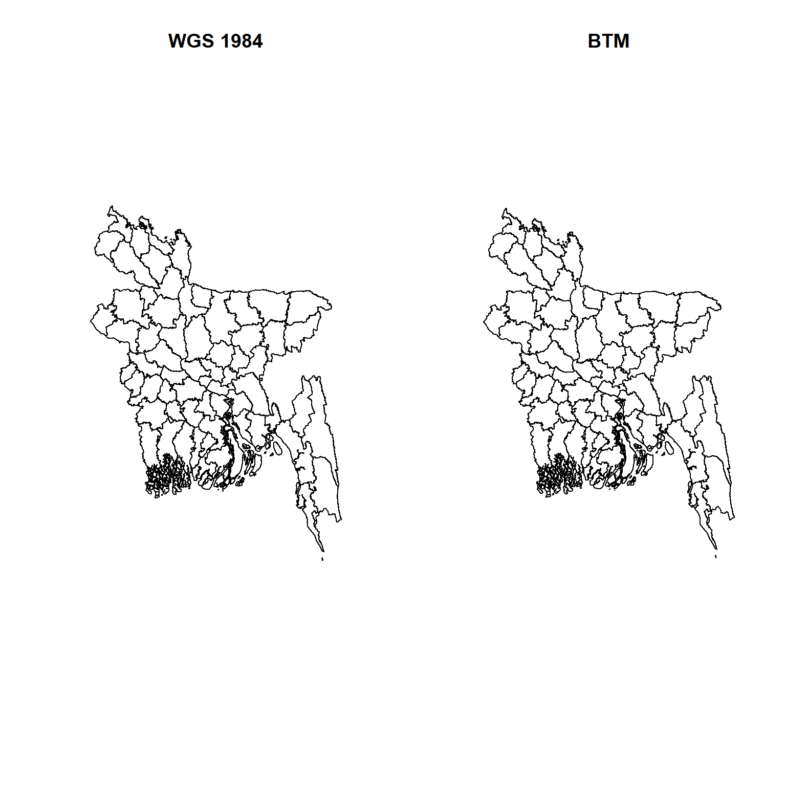
We will transform the shape file to Bangladesh Transverse Mercator (EPSG:9677)
Projection parameter of Bangladesh Transverse Mercator
Object of class SpatialPolygonsDataFrame
Coordinates:
       min      max
x 298487.8 778101.8
y 278578.1 946939.2
Is projected: TRUE
proj4string :
[+proj=tmerc +lat_0=0 +lon_0=90 +k=0.9996 +x_0=500000 +y_0=-2000000
+datum=WGS84 +units=m +no_defs]
Data attributes:
   Shape_Leng       Shape_Area       ADM2_EN           ADM2_PCODE
 Min.   : 1.743   Min.   :0.0623   Length:64          Length:64
 1st Qu.: 2.672   1st Qu.:0.1171   Class :character   Class :character
 Median : 3.581   Median :0.1768   Mode  :character   Mode  :character
 Mean   : 4.331   Mean   :0.1937
 3rd Qu.: 4.821   3rd Qu.:0.2416
 Max.   :13.381   Max.   :0.5070
   ADM2_REF          ADM2ALT1EN         ADM2ALT2EN          ADM1_EN
 Length:64          Length:64          Length:64          Length:64
 Class :character   Class :character   Class :character   Class :character
 Mode  :character   Mode  :character   Mode  :character   Mode  :character


  ADM1_PCODE          ADM0_EN           ADM0_PCODE            date
 Length:64          Length:64          Length:64          Length:64
 Class :character   Class :character   Class :character   Class :character
 Mode  :character   Mode  :character   Mode  :character   Mode  :character


   validOn            ValidTo
 Length:64          Length:64
 Class :character   Class :character
 Mode  :character   Mode  :character
We notice that x and y -coordinates converted from degree-decimal to meter and Is projected: TRUE.
Or we can also use st_transform to st object to project the vector data
Code
# change CRS using st_transformdist.st=sf::st_read(paste0(dataFolder, "/Shapefiles/bd_district_GCS.shp")) # read polygon
Reading layer `bd_district_GCS' from data source
  `G:\My Drive\Data\Bangladesh\Shapefiles\bd_district_GCS.shp'
  using driver `ESRI Shapefile'
Simple feature collection with 64 features and 14 fields
Geometry type: MULTIPOLYGON
Dimension:     XY
Bounding box:  xmin: 88.00863 ymin: 20.59061 xmax: 92.68031 ymax: 26.63451
Geodetic CRS:  GCS_unknown
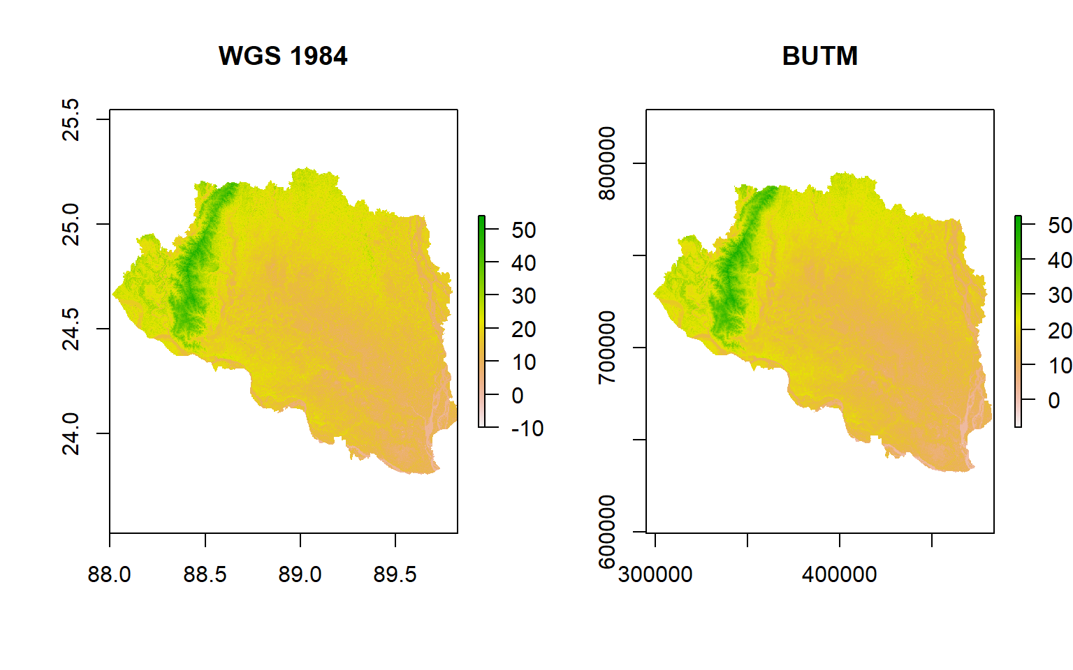
First, we will re-project DEM raster data from WGS 1984 CRS to BUTM projection system. You can load DEM raster in R using raster() function of raster package. If you want to check raster attribute, just simple type r-object name of this raster or use crs() function.
You notice that CRS of this DEM has already been defined as WGS 84. Now, we will project from WGS 84 to BTM. We will use projectRaster() function with proj.4 projection description of BTM ( btm=’ +proj=tmerc +lat_0=0 +lon_0=90 +k=0.9996 +x_0=500000 +y_0=-2000000 +datum=WGS84 +units=m +no_defs’) Be patient, it will take a while to project this DEM data.
Now we will save this projected raster using writeRaster() function of raster package
Code
writeRaster(DEM.PROJ, # Input rasterpaste0(dataFolder,"Raster/raj_DEM_BUTM.tif"), # output folder and output raster"GTiff", # output raster file extensionoverwrite=TRUE) # write on existing file, if exist
Batch Projection of Multiple Raster
In this exercise will project DEM raster of eight divisions in a loop. First, we will create a list of raster using list.files() function and then will create output raster using gsub() function
[{fig-align="left" width="200"}](https://github.com/zia207/r-colab/blob/main/map_projection_coordinate_ref.ipynb)# Map Projection and Coordinate Reference Systems in R {.unnumbered}## Coordinate Reference SystemsCoordinate Reference Systems (CRS) are used in cartography, geography, and GIS (Geographic Information Systems) to define the positions of points, lines, and areas on the Earth's surface. A CRS provides a framework for translating geographic locations, which are expressed as latitude and longitude or other coordinate values, into a specific location on a map or a two-dimensional plane.There are two main types of Coordinate Reference Systems:1. Geographic Coordinate Systems (GCS): Geographic Coordinate Systems use latitude and longitude to define locations on the Earth's surface. Latitude measures the north-south position, while longitude measures the east-west position. The coordinates are expressed in degrees, minutes, and seconds or decimal degrees. Common GCS examples include WGS 84 (World Geodetic System 1984) and NAD83 (North American Datum 1983).2. Projected Coordinate Systems (PCS): Projected Coordinate Systems use Cartesian coordinates (X, Y) to represent locations on a flat, two-dimensional map. The projection converts the three-dimensional geographic coordinates (latitude, longitude, and often elevation) into these two-dimensional coordinates. Different map projections, such as Mercator, Robinson, or UTM (Universal Transverse Mercator), create projected coordinate systems.[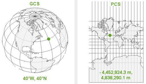](https://pro.arcgis.com/en/pro-app/latest/help/mapping/properties/coordinate-systems-and-projections.htm)Source: ESRIThe equidistant lines that run east and west each have a constant latitude value called **parallels**. The **equator** is the largest circle and divides the earth in half. It is equal in distance from each of the poles, and the value of this latitude line is zero. Locations north of the equator has positive latitudes that range from **0 to +90 degrees**, while locations south of the equator have negative latitudes that range from **0 to -90 degrees**.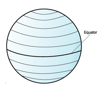{width="236"}The lines that run through north and south each have a constant longitude value and form circles of the same size around the earth known as **meridians**. The **prime meridian** is the line of longitude that defines the origin (zero degrees) for longitude coordinates. One of the most commonly used prime meridian locations is the line that passes through Greenwich, England. Locations east of the prime meridian up to its antipodal meridian (the continuation of the prime meridian on the other side of the globe) have positive longitudes ranging from **0 to +180 degrees**. Locations west of the prime meridian has negative longitudes ranging from **0 to -180 degrees**.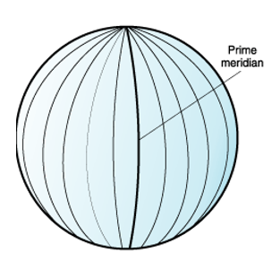{width="256"}The latitude and longitude lines cover the globe to form a grid that know as a **graticule**. The point of origin of the graticule is (0,0), where the equator and the prime meridian intersect. The equator is the only place on the graticule where the linear distance corresponding to one degree latitude is approximately equal the distance corresponding to one degree longitude. Because the longitude lines converge at the poles, the distance between two meridians is different at every parallel.To maintain accuracy in GIS and cartographic applications, it's essential to use the appropriate coordinate reference system and datum for the specific region or project. Choosing the wrong CRS can lead to distortions and inaccuracies when transforming between geographic locations and map coordinates.CRS is a fundamental aspect of spatial data management, as they allow for the integration of different data sources, analysis, and visualization of geographic information consistently and meaningfully. Understanding CRS is crucial for cartographers, GIS analysts, and anyone working with geographic data to ensure accurate spatial representation and analysis.## Map ProjectionMap projection is a method used to represent the three-dimensional surface of the Earth on a two-dimensional map. Since the Earth is a spherical object, it is challenging to depict its curved surface accurately on a flat surface. This problem arises because representing the entire curved surface of the Earth on a flat map results in distortions in shape, size, distance, or direction.Various map projections are available, each designed to address different needs and minimize certain types of distortion. Here are some common types of map projections:Mercator Projection: Developed by Gerardus Mercator in the 16th century, this projection preserves straight lines, making it useful for marine navigation. However, it distorts the sizes of landmasses, with areas near the poles appearing significantly more significant than they are.Robinson Projection: This compromise projection attempts to balance size, shape, and distance distortions across the entire map. It's commonly used for world maps.Conic Projection: This projection involves projecting the Earth's surface onto a cone and then unrolling the cone to form a flat map. It preserves shapes and distances well within the cone area but can have significant distortions as one moves away from that central area.Cylindrical Projection: This projection wraps the Earth's surface around a cylinder. Examples include the Mercator projection mentioned earlier and the Miller projection, which preserves relative size but distorts shapes.Azimuthal Projection: These projections project the Earth's surface onto a plane from a specific point on the Earth's surface. They preserve directionality but can have considerable distortions in other aspects.Goode's Homolosine Projection: This projection combines the sinusoidal and Mollweide projection to reduce landmass size distortion, although it sacrifices shape accuracy.The choice of map projection depends on the intended use of the map, the area being represented, and the extent to which certain distortions are acceptable. No single projection can perfectly represent the entire Earth without any distortions, and mapmakers must make trade-offs based on their specific needs.It's important to understand that map projections are just one aspect of cartography, and producing accurate and valuable maps often involves other techniques, such as generalization, symbolization, and labeling.{{< video https://youtu.be/nJ5r4HJMrfo >}}source: \[LizardTech University\](https://www.youtube.com/\@lizardtechuniversity4210)## The World Geodetic system 84The World Geodetic System 1984 (WGS 84) is a global geodetic reference system developed and maintained by the United States Department of Defense (DoD). It is widely used as the standard coordinate reference system for the Earth's surface in various applications, including mapping, navigation, surveying, and GPS (Global Positioning System).WGS 84 is an Earth-centered, Earth-fixed coordinate system known as a geocentric coordinate system. It defines a three-dimensional model of the Earth, where the center of the Earth serves as the origin, and the X, Y, and Z axes are oriented with respect to the Earth's rotation and equator.The key features of WGS 84 include:1. Ellipsoid: WGS 84 uses the WGS 84 ellipsoid, a mathematically defined surface approximating the shape of the Earth. It is an oblate spheroid, slightly flattened at the poles and bulging at the equator.2. Datum: WGS 84 defines a specific datum, which includes the ellipsoid's size, shape, and orientation in relation to the Earth's center. The datum is a reference frame for measuring positions on the Earth's surface.3. Coordinate Units: WGS 84 uses degrees of latitude and longitude to express geographic positions. Latitude measures the north-south position, and longitude measures the east-west position.4. GPS Reference Frame: WGS 84 is the coordinate system used by the Global Positioning System (GPS). GPS receivers use WGS 84 to accurately determine the user's position on the Earth's surface.5. Constantly Updated: The WGS 84 reference frame is continuously refined and updated to account for crustal movements, which can affect the Earth's shape and position. As such, newer versions of WGS 84 have been released, with slight adjustments to improve accuracy.The adoption of WGS 84 as a global standard has been instrumental in enabling accurate navigation, mapping, and geospatial data exchange across the world. It ensures consistency and interoperability among different mapping and navigation systems, making it possible to integrate data from various sources into a coherent spatial framework.**The parameters of WGS84:**```{r}# GEOGCS["WGS 84", # DATUM["WGS_1984", # SPHEROID["WGS 84",6378137,298.257223563, # AUTHORITY["EPSG","7030"]], # AUTHORITY["EPSG","6326"]], # PRIMEM["Greenwich",0, # AUTHORITY["EPSG","8901"]], # UNIT["degree",0.01745329251994328, # AUTHORITY["EPSG","9122"]], # AUTHORITY["EPSG","4326"]] ```## Universal Transverse Mercator (UTM)The Universal Transverse Mercator (UTM) is a widely used map projection and coordinate reference system that divides the Earth's surface into a series of zones, each with its own unique coordinate system. It is designed to minimize distortion within each zone, making it suitable for accurate mapping and navigation in relatively small areas.The UTM projection is a type of cylindrical projection that projects the Earth's surface onto a cylinder. The cylinder is then unwrapped to create a flat map. The key features of the UTM system include:1. Zone System: The Earth is divided into 60 longitudinal zones, each spanning 6 degrees of longitude. Each zone is 6 degrees wide, except for zones 1 and 60 around the poles, which are narrower to account for the convergence of meridians. Zones are numbered from 1 to 60, starting at the 180° meridian and progressing eastward.2. Transverse Projection: Unlike the Mercator projection, which is based on a standard parallel, the UTM projection is transverse, meaning that the cylinder is oriented along the meridians rather than the equator. This results in better accuracy for regions closer to the equator.3. Cartesian Coordinates: Each UTM zone's positions are expressed in a Cartesian coordinate system with X and Y values. The X-coordinate represents easting (measured in meters) from the central meridian of the zone, and the Y-coordinate represents northing (also measured in meters) from the equator. The origin of each zone is set at the equator and the central meridian of the zone, providing a local reference system.4. False Easting and Northing: To ensure that all coordinates within a zone are positive, a false easting value (500,000 meters) is added to all X-coordinates, and a false northing value is added to all Y-coordinates. This creates a smooth coordinate system without negative values, simplifying calculations.5. Scale Factor: UTM uses a varying scale factor along the central meridian of each zone to further minimize distortion. The scale factor is set to 0.9996, meaning that distances measured on the map are slightly shorter than the actual distances on the Earth's surface.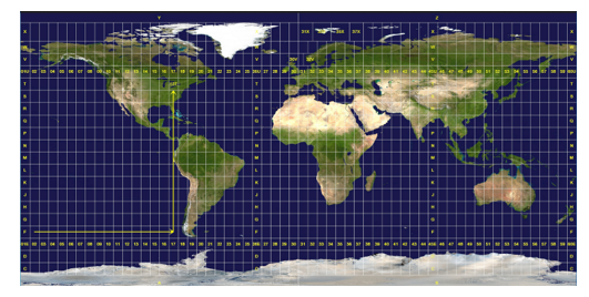The Bangladesh falls in zone 45N (EPSG1:32645) and zone 46N (EPSG:32646).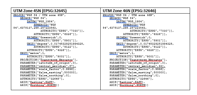{width="549"}UTM is widely used in various applications, including topographic mapping, GPS navigation, military operations, and geospatial data analysis. It is particularly useful for local mapping tasks, covering areas up to a few thousand kilometers in extent, where the distortion is generally kept within acceptable limits. However, it may not be suitable for global maps or large-scale mapping that requires extremely precise measurements over very large areas.### Projection formatThe **PROJ.4** format is a widely used and standardized way of defining the projection and coordinate system parameters for geospatial data. It is employed in many geospatial software libraries and applications to specify how to transform coordinates from one coordinate system to another, or to perform various geospatial operations accurately.The PROJ.4 format consists of a set of parameters, where each parameter represents a specific aspect of the coordinate system or projection. The format is typically represented as a single string with key-value pairs. The basic structure of the PROJ.4 format is as follows:> +proj=<projection> +datum=<datum> +units=<units> +<other_parameters>Here is an explanation of some of the key parameters:1. **`+proj`**: This parameter specifies the projection method or algorithm used to transform coordinates. For example, **`+proj=utm`** for Universal Transverse Mercator, or **`+proj=latlong`** for the WGS84 geographic coordinate system.2. **`+datum`**: This parameter defines the geodetic datum used for the coordinate system. It determines the position of the coordinate system relative to the Earth's ellipsoid. Examples include **`+datum=WGS84`** or **`+datum=NAD83`**.3. **`+units`**: This parameter specifies the units of measurement used in the coordinate system. Common examples include **`+units=meters`** or **`+units=degrees`**.4. **`+other_parameters`**: Additional parameters may be included based on the specific needs of the coordinate system or projection. These parameters can control various aspects, such as false eastings/northings, central meridians, scale factors, etc.Here's an example of the PROJ.4 format for a typical WGS84 Web Mercator (EPSG:3857) and UTM Zone 45 and 46 projection:> +proj=merc +datum=WGS84 +units=meters +no_defs> +proj=utm +zone=45 +datum=WGS84 +units=m +no_defs +type=crs> +proj=utm +zone=46 +datum=WGS84 +units=m +no_defs +type=crs### Load R-packages```{r}#|warning:false#|error:falselibrary(raster) library (rgdal)library(sf)library(maptools)```### DataIn this exercise, we will learn how to check and define CRS and projection of **vector** and **raster** data in R. This is a very important step for working with geospatial data with different projection systems from different sources. We will use following data set:1. Spatial polygon of the district of Bangladesh (bd_district.shp) 2. SRTM DEM raster of Rajshahi division (raj_DEM_GCS.tif)3. One tile of Landsat 9 for Rajshahi DivisionAll data could be found [here](https://github.com/zia207/r-colab/tree/main/Data/Bangladesh/) for download.## Coordinate Reference System of Vector dataWe will use bd_district shape files to check, define projection. We will use **shapefile()** function of raster package to load Vector data in R.```{r}#| warning: false#| error: falsedataFolder<-"G:\\My Drive\\Data\\Bangladesh\\"# if data in working directorydist<-raster::shapefile(paste0(dataFolder, "/Shapefiles/bd_district.shp")) ```### Check ProjectionWe can check current CRS of dist.CGS objects using proj4string() function:```{r}#| warning: false#| error: falseprint(proj4string(dist))```You notice that **.prj** file is not associated with this shape file.We know that bd_district.shp file is in geographic coordinate system. We can also check it coordinates system with **summary()** function.```{r}#| warning: false#| error: falsesummary(dist)```### Define CRSYou notice that county shape file read as **SpatialPolygonsDataFrame** in R, and it's x-coordinate is from 88.00863 to 89.82498 and y-cordinate 23.80807 to 25.27759 and CRS has not been be defined yet (**Is projected: NA and proj4string : \[NA\]**) and **.PRJ** file is missing. So you need to define its current CRS (**WGS 1984 or EPSG:4326**) before you do any further analyses like re-projection etc.We use either of following function to define it's CRS.```{r}#| warning: false#| error: falseproj4string(dist) =CRS("+proj=longlat +ellps=WGS84")# or#proj4string(dist.GCS) <- CRS("+init=epsg:4326")```A new CRS, **WGS 1984** has been assigned to the shape file. You can check it again with **st_crs()** functions.```{r}#| warning: false#| error: falsest_crs(dist)#str(county.GCS)```However, you need to save the file to make it permanent. You can use either, will use **writeOGR()** function of **rgdal** package or **shapefile()** function of raster package or **st_write()** function of **sf** to save it. It is a good practice to write a file with it's current CRS. After running this function, you can see a file named **bd_district_GCS.prj** has created in your working directory.```{r}#| warning: false#| error: falseshapefile(dist, paste0(dataFolder,"shapefiles/bd_district_GCS.shp"), overwrite=TRUE)```### ProjectionThe **spTransform** function provides transformation between datum(s) and conversion between projections (also known as projection and/or re-projection) from one specified coordinate reference system to another. For simple projection, when no **+datum** tags are used, datum projection does not occur. When datum transformation is required, the **+datum** tag should be present with a valid value both in the CRS of the object to be transformed, and in the target CRS. In general **+datum=** is to be preferred to **+ellps=**, because the datum always fixes the ellipsoid, but the ellipsoid never fixes the datum.We will transform the shape file to Bangladesh Transverse Mercator [(EPSG:9677)](https://epsg.io/9677)Projection parameter of Bangladesh Transverse Mercator> "proj=tmerc +lat_0=0 +lon_0=90 +k=0.9996 +x_0=500000 +y_0=-2000000 +datum=WGS84 +units=m +no_defs"```{r}#| warning: false#| error: falsebtm =CRS("+proj=tmerc +lat_0=0 +lon_0=90 +k=0.9996 +x_0=500000 +y_0=-2000000 +datum=WGS84 +units=m +no_defs")# define new projectiondist.PROJ<-spTransform(dist, btm)summary(dist.PROJ)```We notice that x and y -coordinates converted from degree-decimal to meter and **Is projected: TRUE**.Or we can also use st_transform to st object to project the vector data```{r}#| warning: false#| error: false# change CRS using st_transformdist.st=sf::st_read(paste0(dataFolder, "/Shapefiles/bd_district_GCS.shp")) # read polygonst_transform(dist.st, crs=btm)```Now plot WWGS 1984 and BTM projected map site by site.```{r}#| warning: false#| error: false#| fig.width: 8#| fig.height: 8par(mfrow=c(1,2))plot(dist, main="WGS 1984")plot(dist.PROJ, main="BTM")par(mfrow=c(1,1))```We can save (write) this file as an ESRI shape with **writeOGR()** or **shapefile()** or **st_write()** function for future use.```{r,collapse = TRUE}#raster::shapefile(dist.PROJ, paste0(dataFolder,"/Shapefiles/bd_district_BTM.shp"),overwrite=TRUE)```## Raster Data ### Projection of a Single RasterFirst, we will re-project DEM raster data from WGS 1984 CRS to BUTM projection system. You can load DEM raster in R using **raster()** function of **raster** package. If you want to check raster attribute, just simple type r-object name of this raster or use **crs()** function.```{r,fig.align='center',collapse = TRUE}DEM.GCS<-raster::raster(paste0(dataFolder,"/Raster/raj_DEM_GCS.tif"))DEM.GCS# Orcrs(DEM.GCS)```You notice that CRS of this DEM has already been defined as **WGS 84**. Now, we will project from **WGS 84** to **BTM**. We will use **projectRaster()** function with proj.4 projection description of **BTM** ( btm=' +proj=tmerc +lat_0=0 +lon_0=90 +k=0.9996 +x_0=500000 +y_0=-2000000 +datum=WGS84 +units=m +no_defs') Be patient, it will take a while to project this DEM data.```{r message=F, warning=F,fig.align='center'}DEM.PROJ<-projectRaster(DEM.GCS, crs=btm) DEM.PROJ``````{r,echo=TRUE, fig.align='center',fig.height=5, fig.width=8}par(mfrow=c(1,2))plot(DEM.GCS, main="WGS 1984")plot(DEM.PROJ, main="BUTM")par(mfrow=c(1,1))```Now we will save this projected raster using **writeRaster()** function of raster package```{r}writeRaster(DEM.PROJ, # Input rasterpaste0(dataFolder,"Raster/raj_DEM_BUTM.tif"), # output folder and output raster"GTiff", # output raster file extensionoverwrite=TRUE) # write on existing file, if exist ```### Batch Projection of Multiple RasterIn this exercise will project DEM raster of eight divisions in a loop. First, we will create a list of raster using **list.files()** function and then will create output raster using **gsub()** function```{r,collapse = TRUE}# Input raster listDEM.input <-list.files(path=paste0(dataFolder,".//Raster//BD_DEM//GCS"),pattern='.tif$',full.names=T) DEM.input``````{r,collapse = TRUE}# Output raster names DEM.output <-gsub("\\.tif$", "_PROJ.tif", DEM.input) DEM.output```We will define proj.4 projection description of **BTM** as a mew projection and run **projectRaster()** function in a loop```{r message=F, warning=F}# Define a new projectionnewproj <-"+proj=tmerc +lat_0=0 +lon_0=90 +k=0.9996 +x_0=500000 +y_0=0 +datum=WGS84 +units=m +no_defs"# Reprojection and write rasterfor (i in1:8){ r <-raster(DEM.input[i]) PROJ <-projectRaster(r, crs=newproj, method ='bilinear', filename = DEM.output[i], overwrite=TRUE)}```### Further Reading1. [Using map projections](https://cran.r-project.org/web/packages/oce/vignettes/D_map_projections.html)2. [Map Projections in R](https://michaelminn.net/tutorials/r-projections/index.html)3. [Variations on map projections in R](https://www.happykhan.com/posts/map-projections-in-r/)