Code
library(gbm)Gradient Boosting Machine (GBM) is a powerful and popular supervised learning algorithm used for both regression and classification tasks. It belongs to the family of ensemble methods, which combine multiple weak learners to form a stronger model. The idea behind gradient boosting is to iteratively improve a model’s predictions by fitting a new model to the residuals or errors of the previous models.
Whereas random forests build an ensemble of deep independent trees, GBMs build an ensemble of shallow and weak successive trees with each tree learning and improving on the previous. When combined, these many weak successive trees produce a powerful “committee” that are often hard to beat with other algorithms.
The main idea of boosting is to add new models to the ensemble sequentially. At each particular iteration, a new weak, base-learner model is trained with respect to the error of the whole ensemble learnt so far.
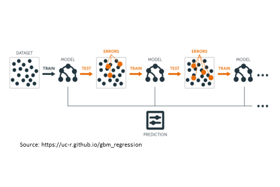
Here’s how GBM works:
Initially, a simple model is fitted to the data. This can be any model such as a decision tree, linear regression, or logistic regression.
The model’s predictions are compared with the actual values of the target variable, and the errors or residuals are calculated.
A new model is then fitted to these residuals, with the aim of reducing the errors made by the first model. The new model is usually a decision tree, but can also be another type of model.
The predictions of this new model are added to the predictions of the previous model, and the errors are recalculated.
Steps 3 and 4 are repeated iteratively, with each new model attempting to reduce the errors of the previous model. The final predictions are the sum of the predictions of all the models.
To avoid overfitting, the model can be regularized by adding constraints on the size or complexity of the trees, or by using early stopping.
Gradient boosting has several advantages over other methods, such as its ability to handle different types of data (e.g. numerical, categorical), its robustness to outliers and noise, and its high accuracy on many problems. However, it can also be computationally expensive and sensitive to hyperparameters, such as the learning rate, the number of trees, and the depth of the trees.
Random Forest (RF) and Gradient Boosting Machine (GBM) are both popular ensemble methods used for supervised learning tasks. While they share some similarities, there are several key differences between the two algorithms:
Sampling approach: RF builds multiple decision trees on randomly sampled subsets of the data with replacement, while GBM builds trees sequentially on the residuals or errors of the previous trees.
Learning process: RF trees are built independently, while GBM trees are built in a sequential manner, with each new tree attempting to improve upon the errors of the previous trees.
Bias-variance tradeoff: RF tends to have a lower variance and higher bias, while GBM tends to have a lower bias and higher variance.
Model interpretability: RF is generally more interpretable, as the feature importances can be easily calculated based on the frequency of their use in the trees. GBM, on the other hand, can be more challenging to interpret, as the importance of each feature depends on the interaction with other features and the specific stage of the boosting process.
Performance: Both RF and GBM can perform well on a wide range of problems, but their performance may depend on the specific characteristics of the data and the problem at hand.
In general, RF may be a good choice for problems where model interpretability is important, or where there are many noisy or irrelevant features. GBM may be a good choice for problems where high accuracy is desired, and where the data has complex interactions between features. However, the choice between RF and GBM ultimately depends on the specific characteristics of the problem and the goals of the analysis.
The gbm R package is an implementation of extensions to Freund and Schapire’s AdaBoost algorithm and Friedman’s gradient boosting machine. This is the original R implementation of GBM.
To get started with the gbm package, you can install it from CRAN using the following code:
install.packages(“gbm”)
library(gbm)In this exercise we will use following data se and use DEM, MAP, MAT, NAVI, NLCD, and FRG to fit a GBM regression model.
library(tidyverse)
# define data folder
dataFolder<-"E:/Dropbox/GitHub/Data/USA/"
# Load data
mf<-read_csv(paste0(dataFolder, "gp_soil_data.csv"))
# Create a data-frame
df<-mf %>% dplyr::select(SOC, DEM, Slope, Aspect, TPI, KFactor, SiltClay, MAT, MAP,NDVI, NLCD, FRG)%>%
    glimpse()
Rows: 467
Columns: 12
$ SOC <dbl> 15.763, 15.883, 18.142, 10.745, 10.479, 16.987, 24.954, 6.288…
$ DEM <dbl> 2229.079, 1889.400, 2423.048, 2484.283, 2396.195, 2360.573, 2…
$ Slope <dbl> 5.6716146, 8.9138117, 4.7748051, 7.1218114, 7.9498644, 9.6632…
$ Aspect <dbl> 159.1877, 156.8786, 168.6124, 198.3536, 201.3215, 208.9732, 2…
$ TPI <dbl> -0.08572358, 4.55913162, 2.60588670, 5.14693117, 3.75570583, …
$ KFactor <dbl> 0.31999999, 0.26121211, 0.21619999, 0.18166667, 0.12551020, 0…
$ SiltClay <dbl> 64.84270, 72.00455, 57.18700, 54.99166, 51.22857, 45.02000, 5…
$ MAT <dbl> 4.5951686, 3.8599243, 0.8855000, 0.4707811, 0.7588266, 1.3586…
$ MAP <dbl> 468.3245, 536.3522, 859.5509, 869.4724, 802.9743, 1121.2744, …
$ NDVI <dbl> 0.4139390, 0.6939532, 0.5466033, 0.6191013, 0.5844722, 0.6028…
$ NLCD <chr> "Shrubland", "Shrubland", "Forest", "Forest", "Forest", "Fore…
$ FRG <chr> "Fire Regime Group IV", "Fire Regime Group IV", "Fire Regime …df$NLCD <- as.factor(df$NLCD)
df$FRG <- as.factor(df$FRG)We use rsample package, install with tidymodels, to split data into training (70%) and test data (30%) set with Stratified Random Sampling. initial_split() creates a single binary split of the data into a training set and testing set.
Stratified random sampling is a technique for selecting a representative sample from a population, where the sample is chosen in a way that ensures that certain subgroups within the population are adequately represented in the sample.
#
#| fig.width: 4
#| fig.height: 4

library(tidymodels)
set.seed(1245)   # for reproducibility
split <- initial_split(df, prop = 0.8, strata = SOC)
train <- split %>% training()
test <-  split %>% testing()

# Density plot all, train and test data
ggplot()+
  geom_density(data = df, aes(SOC))+
  geom_density(data = train, aes(SOC), color = "green")+
  geom_density(data = test, aes(SOC), color = "red") +
      xlab("Soil Organic Carbon (kg/g)") +
ylab("Density") 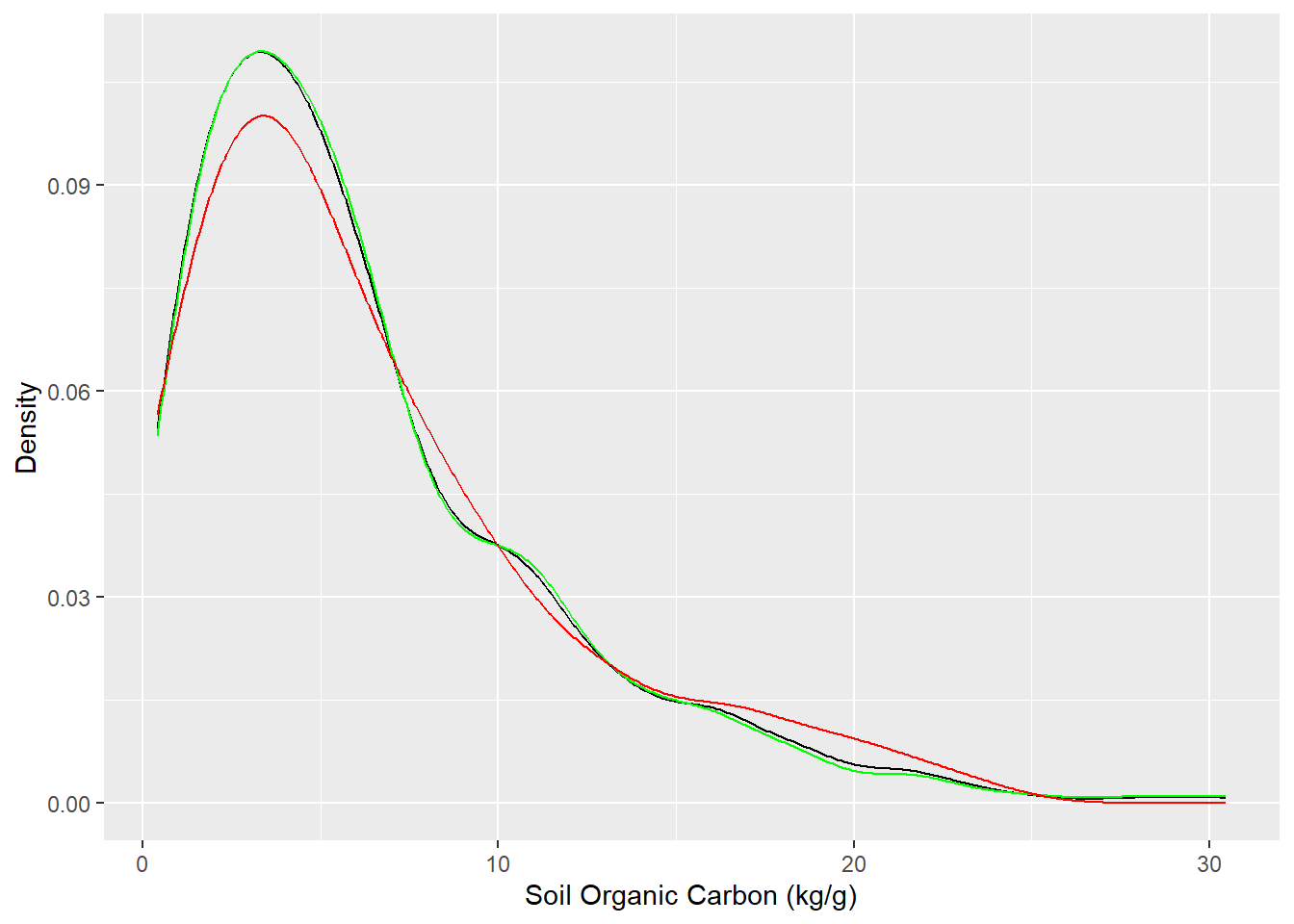
train[-c(1, 11,12)] = scale(train[-c(1,11,12)])
test[-c(1, 11,12)] = scale(test[-c(1,11,12)])We will fit a tree-based GBM model with a few parameters using gbm() function:
set.seed(123)
# train GBM model
gbm.fit <- gbm(
          formula = SOC ~ .,
          data = train,             # dataframe
          distribution = "gaussian",# a character string specifying  data distribution
          n.trees = 5000,           #  the total number of trees to fit,
                                    # default 100
          interaction.depth = 1,    # maximum depth of each tree
                                    # A value of 1 implies an additive model,
                                    # a value of 2 implies a model with up to 2-way interactions, etc.
                                    # Default is 1
          shrinkage = 0.001,        # a shrinkage parameter applied to each tree in the expansion.
                                    # Also known as the learning rate or step-size reduction;
                                    # 0.001 to 0.1 usually work,
                                    # but a smaller learning rate typically requires more trees.
                                    # Default is 0.1.
          bag.fraction = 0.7,       # the fraction of the training set observations randomly selected
                                    # to propose the next tree in the expansion.
                                    # This introduces randomnesses into the model fit.
                                    # If bag.fraction < 1 then running the same model twice
                                    # will result in similar but different fits.
                                    # gbm uses the R random number generator so set.seed
                                    # can ensure that the model can be reconstructed.
                                    # Preferably, the user can save the returned gbm.object using save.
                                    # Default is 0.5
          cv.folds = 5,             # cross-validation folds
          n.cores = NULL,           # will use all cores by default
          verbose = F           # Logical indicating whether or not to print out progress and performance indicators (TRUE)
) gbm.fitgbm(formula = SOC ~ ., distribution = "gaussian", data = train,
n.trees = 5000, interaction.depth = 1, shrinkage = 0.001,
bag.fraction = 0.7, cv.folds = 5, verbose = F, n.cores = NULL)
A gradient boosted model with gaussian loss function.
5000 iterations were performed.
The best cross-validation iteration was 4999.
There were 11 predictors of which 11 had non-zero influence.# get MSE and compute RMSE
sqrt(min(gbm.fit$cv.error))[1] 4.048704Estimates the optimal number of boosting iterations for a gbm object and optionally plots various performance measures
gbm.perf(gbm.fit, method = "cv")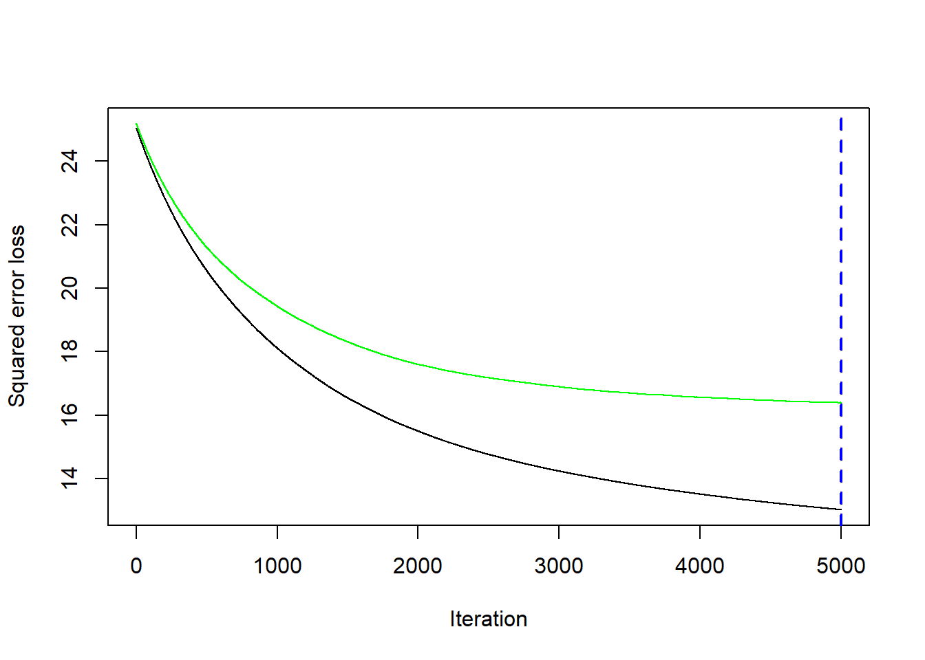
[1] 4999test$SOC.pred = predict(gbm.fit, newdata = test)library(Matrix)
RMSE<- Metrics::rmse(test$SOC, test$SOC.pred)
RMSE[1] 3.55045library(ggpmisc)
formula<-y~x
ggplot(test, aes(SOC,SOC.pred)) +
geom_point() +
geom_smooth(method = "lm")+
stat_poly_eq(use_label(c("eq", "adj.R2")), formula = formula) +
ggtitle("Gradient Boosting Machine (GBM)") +
xlab("Observed") + ylab("Predicted") +
scale_x_continuous(limits=c(0,25), breaks=seq(0, 25, 5))+
scale_y_continuous(limits=c(0,25), breaks=seq(0, 25, 5)) +
# Flip the bars
theme(
panel.background = element_rect(fill = "grey95",colour = "gray75",size = 0.5, linetype = "solid"),
axis.line = element_line(colour = "grey"),
plot.title = element_text(size = 14, hjust = 0.5),
axis.title.x = element_text(size = 14),
axis.title.y = element_text(size = 14),
axis.text.x=element_text(size=13, colour="black"),
axis.text.y=element_text(size=13,angle = 90,vjust = 0.5, hjust=0.5, colour='black'))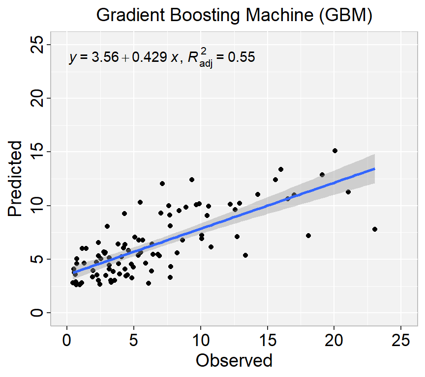
method = relative.influence: At each split in each tree, gbm computes the improvement in the split-criterion (MSE for regression). gbm then averages the improvement made by each variable across all the trees that the variable is used. The variables with the largest average decrease in MSE are considered most important.
method = permutation.test.gbm: For each tree, the OOB sample is passed down the tree and the prediction accuracy is recorded. Then the values for each variable (one at a time) are randomly permuted and the accuracy is again computed. The decrease in accuracy as a result of this randomly “shaking up” of variable values is averaged over all the trees for each variable. The variables with the largest average decrease in accuracy are considered most important.
summary(
  gbm.fit,
  cBars = 10,
  method = relative.influence, # also can use permutation.test.gbm
  las = 2
  )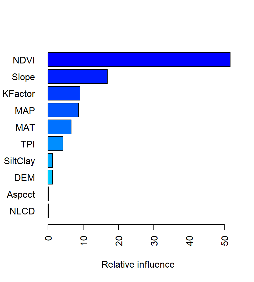
              var     rel.inf
NDVI         NDVI 51.63209061
Slope       Slope 16.82052947
KFactor   KFactor  9.07920252
MAP           MAP  8.68191448
MAT           MAT  6.55400113
TPI           TPI  4.24848710
SiltClay SiltClay  1.33348869
DEM           DEM  1.30516352
Aspect     Aspect  0.16689032
NLCD         NLCD  0.11403561
FRG           FRG  0.06419656
An alternative approach is to use the vip package, which provides ggplot2 plots. vip also provides an additional measure of variable importance based on partial dependence measures and is a common variable importance plotting framework for many machine learning models
library(vip)
vip(gbm.fit)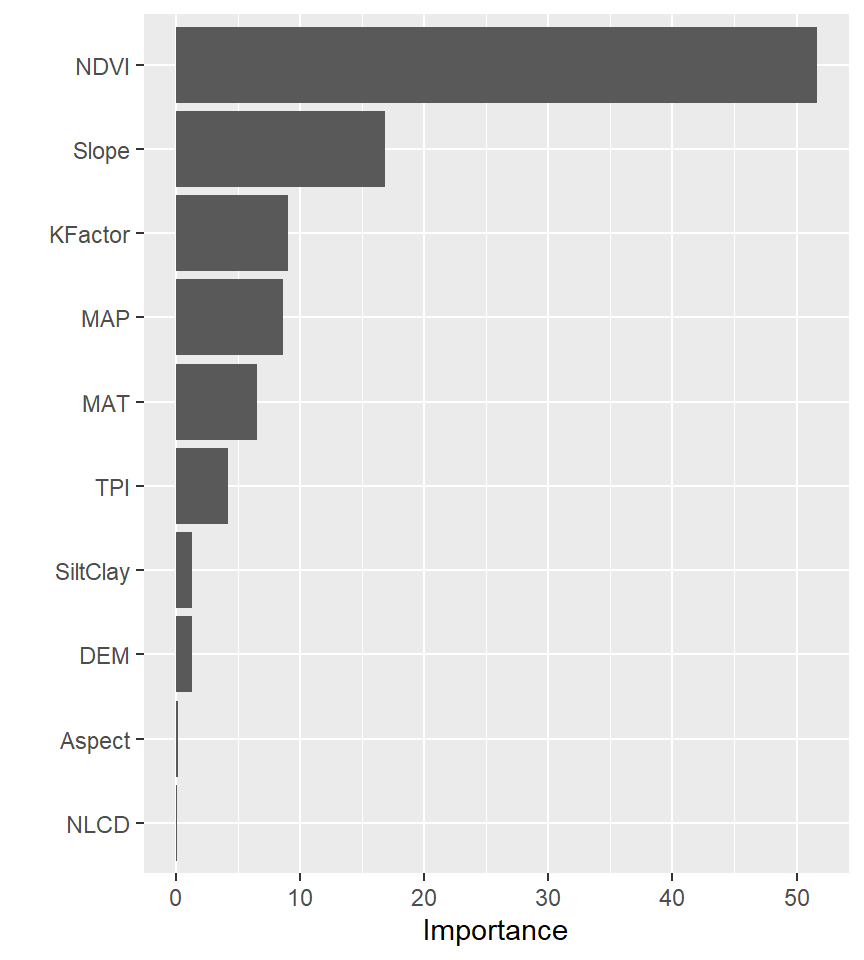
#  remove all object
rm(list = ls())h20 includes an implementation of gradient boosting machine (GBM) that can be used for both regression and classification problems. H2O’s GBM sequentially builds regression trees on all the features of the dataset in a fully distributed way - each tree is built in parallel.
First we will use h2o.gbm() function to build gradient boosted regression trees with some predefined hyper-parameters
library(tidyverse)

# define data folder
dataFolder<-"E:/Dropbox/GitHub/Data/USA/"
# Load data
mf<-read_csv(paste0(dataFolder, "gp_soil_data.csv"))
# Create a data-frame
df<-mf %>% dplyr::select(SOC, DEM, Slope, Aspect, TPI, KFactor, SiltClay, MAT, MAP,NDVI, NLCD, FRG)%>%
    glimpse()
Rows: 467
Columns: 12
$ SOC <dbl> 15.763, 15.883, 18.142, 10.745, 10.479, 16.987, 24.954, 6.288…
$ DEM <dbl> 2229.079, 1889.400, 2423.048, 2484.283, 2396.195, 2360.573, 2…
$ Slope <dbl> 5.6716146, 8.9138117, 4.7748051, 7.1218114, 7.9498644, 9.6632…
$ Aspect <dbl> 159.1877, 156.8786, 168.6124, 198.3536, 201.3215, 208.9732, 2…
$ TPI <dbl> -0.08572358, 4.55913162, 2.60588670, 5.14693117, 3.75570583, …
$ KFactor <dbl> 0.31999999, 0.26121211, 0.21619999, 0.18166667, 0.12551020, 0…
$ SiltClay <dbl> 64.84270, 72.00455, 57.18700, 54.99166, 51.22857, 45.02000, 5…
$ MAT <dbl> 4.5951686, 3.8599243, 0.8855000, 0.4707811, 0.7588266, 1.3586…
$ MAP <dbl> 468.3245, 536.3522, 859.5509, 869.4724, 802.9743, 1121.2744, …
$ NDVI <dbl> 0.4139390, 0.6939532, 0.5466033, 0.6191013, 0.5844722, 0.6028…
$ NLCD <chr> "Shrubland", "Shrubland", "Forest", "Forest", "Forest", "Fore…
$ FRG <chr> "Fire Regime Group IV", "Fire Regime Group IV", "Fire Regime …df$NLCD <- as.factor(df$NLCD)
df$FRG <- as.factor(df$FRG)library(tidymodels)
set.seed(1245) # for reproducibility
split.df <- initial_split(df, prop = 0.8, strata = SOC)
train <- split.df %>% training()
test <- split.df %>% testing()train[-c(1, 11,12)] = scale(train[-c(1,11,12)])
test[-c(1, 11,12)] = scale(test[-c(1,11,12)])library(h2o)
h2o.init(nthreads = -1, max_mem_size = "198g", enable_assertions = FALSE)
H2O is not running yet, starting it now...

Note:  In case of errors look at the following log files:
    C:\Users\zahmed2\AppData\Local\Temp\1\RtmpKStH1N\file7a004dc42c8b/h2o_zahmed2_started_from_r.out
    C:\Users\zahmed2\AppData\Local\Temp\1\RtmpKStH1N\file7a001fc86206/h2o_zahmed2_started_from_r.err


Starting H2O JVM and connecting:  Connection successful!

R is connected to the H2O cluster:
    H2O cluster uptime:         3 seconds 270 milliseconds
    H2O cluster timezone:       America/New_York
    H2O data parsing timezone:  UTC
    H2O cluster version:        3.40.0.4
    H2O cluster version age:    3 months and 23 days
    H2O cluster name:           H2O_started_from_R_zahmed2_qtu738
    H2O cluster total nodes:    1
    H2O cluster total memory:   198.00 GB
    H2O cluster total cores:    40
    H2O cluster allowed cores:  40
    H2O cluster healthy:        TRUE
    H2O Connection ip:          localhost
    H2O Connection port:        54321
    H2O Connection proxy:       NA
    H2O Internal Security:      FALSE
R Version: R version 4.3.1 (2023-06-16 ucrt) #disable progress bar for RMarkdown
h2o.no_progress()
# Optional: remove anything from previous session
h2o.removeAll() h_df=as.h2o(df)
h_train = as.h2o(train)
h_test = as.h2o(test)CV.xy<- as.data.frame(h_train)
test.xy<- as.data.frame(h_test)y <- "SOC"
x <- setdiff(names(h_df), y)gbm_h2o <- h2o.gbm( ## h2o.gbm function
training_frame = h_train, ## the H2O frame for training
# validation_frame = valid, ## the H2O frame for validation (not required)
x=x, ## the predictor columns, by column index
y=y, ## the target index (what we are predicting)
model_id = "GBM_MODEL_IDs", ## name the model in H2O
ntrees = 5000, ## number of trees. Defaults to 50
max_depth =5, ## Maximum tree depth (0 for unlimited). Defaults to 5
min_rows = 8, ## Fewest allowed (weighted) observations in a leaf.
## Defaults to 10.
sample_rate = 0.7, ## Row sample rate per tree (from 0.0 to 1.0) Defaults to 1.
learn_rate = 0.05, ## Learning rate (from 0.0 to 1.0) Defaults to 0.1.
col_sample_rate = 0.6, ## column sample rate (from 0.0 to 1.0) Defaults to 1.
col_sample_rate_per_tree = 0.5, ## Column sample rate per tree (from 0.0 to 1.0) Defaults to 1.
stopping_rounds = 2, ## Stop fitting new trees when the 2-tree
## average is within 0.001 (default) of
## the prior two 2-tree averages.
stopping_metric = "RMSE", ## Metric to use for early stopping
nfolds = 10, ## umber of folds for K-fold cross-validation
## (0 to disable or >= 2). Defaults to 0.
keep_cross_validation_models = TRUE, ## logical. Whether to keep the cross-validation models.
## Defaults to TRUE.
seed = 1000000) ## Set the random seed so that this can be
## reproduced.summary(gbm_h2o)Model Details:
==============
H2ORegressionModel: gbm
Model Key: GBM_MODEL_IDs
Model Summary:
number_of_trees number_of_internal_trees model_size_in_bytes min_depth
1 27 27 6799 5
max_depth mean_depth min_leaves max_leaves mean_leaves
1 5 5.00000 12 20 15.44444
H2ORegressionMetrics: gbm
** Reported on training data. **
MSE: 11.46304
RMSE: 3.385711
MAE: 2.472293
RMSLE: 0.4735253
Mean Residual Deviance : 11.46304
H2ORegressionMetrics: gbm
** Reported on cross-validation data. **
** 10-fold cross-validation on training data (Metrics computed for combined holdout predictions) **

MSE:  16.60818
RMSE:  4.075314
MAE:  2.967318
RMSLE:  0.5453423
Mean Residual Deviance :  16.60818
Cross-Validation Metrics Summary:
mean sd cv_1_valid cv_2_valid cv_3_valid
mae 2.996883 0.459726 3.582629 3.295636 2.700663
mean_residual_deviance 16.886757 6.004311 24.791060 21.579756 11.121973
mse 16.886757 6.004311 24.791060 21.579756 11.121973
r2 0.227871 0.236915 0.241299 0.363155 0.129488
residual_deviance 16.886757 6.004311 24.791060 21.579756 11.121973
rmse 4.052156 0.720177 4.979062 4.645402 3.334962
rmsle 0.540695 0.082977 0.619449 0.505990 0.668331
cv_4_valid cv_5_valid cv_6_valid cv_7_valid cv_8_valid
mae 2.803618 2.376791 2.923173 2.862241 3.860505
mean_residual_deviance 14.661390 13.562562 14.791418 14.795705 27.596037
mse 14.661390 13.562562 14.791418 14.795705 27.596037
r2 0.083854 0.536618 0.295623 0.391947 0.234319
residual_deviance 14.661390 13.562562 14.791418 14.795705 27.596037
rmse 3.829019 3.682738 3.845961 3.846519 5.253193
rmsle 0.417485 0.528491 0.576550 0.457246 0.608179
cv_9_valid cv_10_valid
mae 3.003401 2.560169
mean_residual_deviance 17.274010 8.693666
mse 17.274010 8.693666
r2 0.337826 -0.335414
residual_deviance 17.274010 8.693666
rmse 4.156201 2.948503
rmsle 0.447195 0.578029
Scoring History:
timestamp duration number_of_trees training_rmse training_mae
1 2023-08-20 22:54:28 1.003 sec 0 5.00665 3.78578
2 2023-08-20 22:54:28 1.007 sec 1 4.92158 3.72399
3 2023-08-20 22:54:28 1.011 sec 2 4.84032 3.67325
4 2023-08-20 22:54:28 1.014 sec 3 4.74481 3.58913
5 2023-08-20 22:54:28 1.017 sec 4 4.64259 3.51496
training_deviance
1 25.06656
2 24.22194
3 23.42874
4 22.51320
5 21.55365
---
timestamp duration number_of_trees training_rmse training_mae
23 2023-08-20 22:54:28 1.079 sec 22 3.58764 2.64183
24 2023-08-20 22:54:28 1.081 sec 23 3.53471 2.59816
25 2023-08-20 22:54:28 1.084 sec 24 3.49871 2.56000
26 2023-08-20 22:54:28 1.086 sec 25 3.46543 2.53408
27 2023-08-20 22:54:28 1.089 sec 26 3.42509 2.50455
28 2023-08-20 22:54:28 1.124 sec 27 3.38571 2.47229
training_deviance
23 12.87115
24 12.49419
25 12.24095
26 12.00922
27 11.73124
28 11.46304
Variable Importances: (Extract with `h2o.varimp`)
=================================================
Variable Importances:
variable relative_importance scaled_importance percentage
1 MAP 7498.787598 1.000000 0.159806
2 NDVI 7343.200684 0.979252 0.156490
3 Slope 5935.918945 0.791584 0.126500
4 DEM 4441.913086 0.592351 0.094661
5 KFactor 4251.214355 0.566920 0.090597
6 NLCD 4067.579834 0.542432 0.086684
7 MAT 4000.682373 0.533511 0.085258
8 Aspect 3377.058350 0.450347 0.071968
9 SiltClay 2708.038818 0.361130 0.057711
10 FRG 2278.607178 0.303863 0.048559
11 TPI 1021.276855 0.136192 0.021764# training performance
h2o.performance(gbm_h2o, h_train)H2ORegressionMetrics: gbm
MSE: 11.46304
RMSE: 3.385711
MAE: 2.472293
RMSLE: 0.4735253
Mean Residual Deviance : 11.46304# CV-performance
h2o.performance(gbm_h2o, xval=TRUE)H2ORegressionMetrics: gbm
** Reported on cross-validation data. **
** 10-fold cross-validation on training data (Metrics computed for combined holdout predictions) **
MSE: 16.60818
RMSE: 4.075314
MAE: 2.967318
RMSLE: 0.5453423
Mean Residual Deviance : 16.60818# test performance
h2o.performance(gbm_h2o, h_test)H2ORegressionMetrics: gbm
MSE: 13.28167
RMSE: 3.644403
MAE: 2.712598
RMSLE: 0.545531
Mean Residual Deviance : 13.28167pred.rf <- as.data.frame(h2o.predict(object = gbm_h2o, newdata = h_test))
test_data<-as.data.frame(h_test)
test_data$RF_SOC<-pred.rf$predict We can plot observed and predicted values with fitted regression line with ggplot2
library(ggpmisc)
formula<-y~x

ggplot(test_data, aes(SOC,RF_SOC)) +
  geom_point() +
  geom_smooth(method = "lm")+
  stat_poly_eq(use_label(c("eq", "adj.R2")), formula = formula) +
  ggtitle("H2O-GBM: Observed vs Predicted SOC ") +
  xlab("Observed") + ylab("Predicted") +
  scale_x_continuous(limits=c(0,25), breaks=seq(0, 25, 5))+
  scale_y_continuous(limits=c(0,25), breaks=seq(0, 25, 5)) +
  # Flip the bars
  theme(
    panel.background = element_rect(fill = "grey95",colour = "gray75",size = 0.5, linetype = "solid"),
    axis.line = element_line(colour = "grey"),
    plot.title = element_text(size = 14, hjust = 0.5),
    axis.title.x = element_text(size = 14),
    axis.title.y = element_text(size = 14),
    axis.text.x=element_text(size=13, colour="black"),
    axis.text.y=element_text(size=13,angle = 90,vjust = 0.5, hjust=0.5, colour='black'))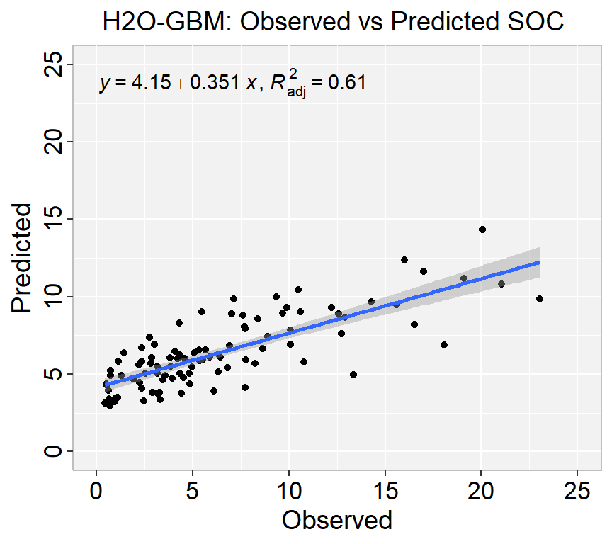
#  remove all object
rm(list = ls())library(tidyverse)
# define data folder
dataFolder<-"E:/Dropbox/GitHub/Data/USA/"
# Load data
mf<-read_csv(paste0(dataFolder, "gp_soil_data.csv"))
# Create a data-frame
df<-mf %>% dplyr::select(SOC, DEM, Slope, Aspect, TPI, KFactor, SiltClay, MAT, MAP,NDVI, NLCD, FRG)%>%
glimpse()Rows: 467
Columns: 12
$ SOC <dbl> 15.763, 15.883, 18.142, 10.745, 10.479, 16.987, 24.954, 6.288…
$ DEM <dbl> 2229.079, 1889.400, 2423.048, 2484.283, 2396.195, 2360.573, 2…
$ Slope <dbl> 5.6716146, 8.9138117, 4.7748051, 7.1218114, 7.9498644, 9.6632…
$ Aspect <dbl> 159.1877, 156.8786, 168.6124, 198.3536, 201.3215, 208.9732, 2…
$ TPI <dbl> -0.08572358, 4.55913162, 2.60588670, 5.14693117, 3.75570583, …
$ KFactor <dbl> 0.31999999, 0.26121211, 0.21619999, 0.18166667, 0.12551020, 0…
$ SiltClay <dbl> 64.84270, 72.00455, 57.18700, 54.99166, 51.22857, 45.02000, 5…
$ MAT <dbl> 4.5951686, 3.8599243, 0.8855000, 0.4707811, 0.7588266, 1.3586…
$ MAP <dbl> 468.3245, 536.3522, 859.5509, 869.4724, 802.9743, 1121.2744, …
$ NDVI <dbl> 0.4139390, 0.6939532, 0.5466033, 0.6191013, 0.5844722, 0.6028…
$ NLCD <chr> "Shrubland", "Shrubland", "Forest", "Forest", "Forest", "Fore…
$ FRG <chr> "Fire Regime Group IV", "Fire Regime Group IV", "Fire Regime …df$NLCD <- as.factor(df$NLCD)
df$FRG <- as.factor(df$FRG)library(tidymodels)
set.seed(1245) # for reproducibility
split.df <- initial_split(df, prop = 0.8, strata = SOC)
train <- split.df %>% training()
test <- split.df %>% testing()train[-c(1, 11,12)] = scale(train[-c(1,11,12)])
test[-c(1, 11,12)] = scale(test[-c(1,11,12)])library(h2o)
h2o.init(nthreads = -1, max_mem_size = "198g", enable_assertions = FALSE) Connection successful!
R is connected to the H2O cluster:
H2O cluster uptime: 10 seconds 859 milliseconds
H2O cluster timezone: America/New_York
H2O data parsing timezone: UTC
H2O cluster version: 3.40.0.4
H2O cluster version age: 3 months and 23 days
H2O cluster name: H2O_started_from_R_zahmed2_qtu738
H2O cluster total nodes: 1
H2O cluster total memory: 198.00 GB
H2O cluster total cores: 40
H2O cluster allowed cores: 40
H2O cluster healthy: TRUE
H2O Connection ip: localhost
H2O Connection port: 54321
H2O Connection proxy: NA
H2O Internal Security: FALSE
R Version: R version 4.3.1 (2023-06-16 ucrt) #disable progress bar for RMarkdown
h2o.no_progress()
# Optional: remove anything from previous session
h2o.removeAll() h_df=as.h2o(df)
h_train = as.h2o(train)
h_test = as.h2o(test)CV.xy<- as.data.frame(h_train)
test.xy<- as.data.frame(h_test)y <- "SOC"
x <- setdiff(names(h_df), y)GBM_hyper_params = list( ntrees = c(100,500, 1000, 5000),
max_depth = c(2,5,8),
min_rows = c(8,10, 12),
learn_rate = c(0.001,0.05,0.06),
sample_rate = c(0.4,0.5,0.6, 0.7),
col_sample_rate = c(0.4,0.5,0.6),
col_sample_rate_per_tree = c(0.4,0.5,0.6))
GBM_hyper_params$ntrees
[1] 100 500 1000 5000
$max_depth
[1] 2 5 8
$min_rows
[1] 8 10 12
$learn_rate
[1] 0.001 0.050 0.060
$sample_rate
[1] 0.4 0.5 0.6 0.7
$col_sample_rate
[1] 0.4 0.5 0.6
$col_sample_rate_per_tree
[1] 0.4 0.5 0.6search_criteria <- list(strategy = "RandomDiscrete",
max_models = 40,
max_runtime_secs = 300,
stopping_tolerance = 0.001,
stopping_rounds = 2,
seed = 42)GBM_grid <- h2o.grid(
algorithm="gbm",
grid_id = "GBM_grid_ID",
x= x,
y = y,
training_frame = h_train,
#validation_frame = h_valid,
distribution ="AUTO",
stopping_metric = "RMSE",
#fold_assignment ="Stratified",
nfolds=5,
keep_cross_validation_predictions = TRUE,
keep_cross_validation_models = TRUE,
hyper_params = GBM_hyper_params,
search_criteria = search_criteria,
seed = 42)# number GBM
length(GBM_grid@model_ids)[1] 31# Get Model ID
GBM_get_grid <- h2o.getGrid("GBM_grid_ID",
sort_by="RMSE",
decreasing=F)
# Get the best RF model
best_GBM <- h2o.getModel(GBM_get_grid@model_ids[[1]])# training performance
h2o.performance(best_GBM, h_train)H2ORegressionMetrics: gbm
MSE: 11.50257
RMSE: 3.391544
MAE: 2.436229
RMSLE: 0.4559464
Mean Residual Deviance : 11.50257# CV-performance
h2o.performance(best_GBM, xval=TRUE)H2ORegressionMetrics: gbm
** Reported on cross-validation data. **
** 5-fold cross-validation on training data (Metrics computed for combined holdout predictions) **
MSE: 15.76155
RMSE: 3.970082
MAE: 2.864454
RMSLE: 0.5191092
Mean Residual Deviance : 15.76155# test performance
h2o.performance(best_GBM, h_test)H2ORegressionMetrics: gbm
MSE: 11.42624
RMSE: 3.380273
MAE: 2.472756
RMSLE: 0.5001688
Mean Residual Deviance : 11.42624test.pred.RF<-as.data.frame(h2o.predict(object = best_GBM, newdata = h_test))
test.xy$GBM_SOC<-test.pred.RF$predictWe can plot observed and predicted values with fitted regression line with ggplot2
library(ggpmisc)
formula<-y~x

ggplot(test.xy, aes(SOC,GBM_SOC)) +
  geom_point() +
  geom_smooth(method = "lm")+
  stat_poly_eq(use_label(c("eq", "adj.R2")), formula = formula) +
  ggtitle("H2O: The Best GBM: Observed vs Predicted SOC ") +
  xlab("Observed") + ylab("Predicted") +
  scale_x_continuous(limits=c(0,25), breaks=seq(0, 25, 5))+
  scale_y_continuous(limits=c(0,25), breaks=seq(0, 25, 5)) +
  # Flip the bars
  theme(
    panel.background = element_rect(fill = "grey95",colour = "gray75",size = 0.5, linetype = "solid"),
    axis.line = element_line(colour = "grey"),
    plot.title = element_text(size = 14, hjust = 0.5),
    axis.title.x = element_text(size = 14),
    axis.title.y = element_text(size = 14),
    axis.text.x=element_text(size=13, colour="black"),
    axis.text.y=element_text(size=13,angle = 90,vjust = 0.5, hjust=0.5, colour='black'))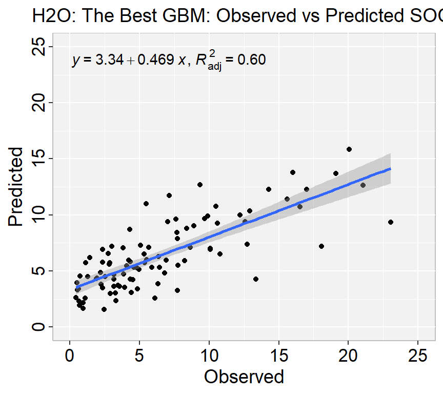
Model explainability refers to the ability to understand and interpret the decisions made by a machine learning model. In other words, it is the ability to explain how a model arrives at its predictions or classifications.
Explainability is particularly important in applications where decisions made by the model have significant real-world consequences, such as in healthcare, finance, and legal fields. It is also important for regulatory compliance, where models must be auditable and transparent.
The h2o.explain() function generates a list of explanations – individual units of explanation such as a Partial Dependence plot or a Variable Importance plot. Most of the explanations are visual – these plots can also be created by individual utility functions outside the h2o.explain() function.
h2o.varimp(best_GBM)Variable Importances:
variable relative_importance scaled_importance percentage
1 NDVI 554005.062500 1.000000 0.247437
2 MAP 408371.750000 0.737126 0.182392
3 Slope 273328.375000 0.493368 0.122078
4 DEM 201504.187500 0.363723 0.089998
5 KFactor 201060.859375 0.362922 0.089800
6 MAT 181140.406250 0.326965 0.080903
7 NLCD 117436.132812 0.211977 0.052451
8 SiltClay 117232.757812 0.211610 0.052360
9 TPI 89372.101562 0.161320 0.039917
10 Aspect 57945.554688 0.104594 0.025880
11 FRG 37576.152344 0.067826 0.016783h2o.varimp_plot(best_GBM)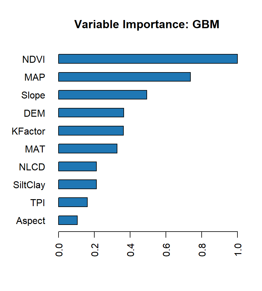
SHAP (SHapley Additive exPlanations) values are a method for explaining the output of any machine learning model. SHAP values provide a way to attribute the prediction of an individual feature to its contribution to the final prediction, taking into account the interaction with other features in the model.
SHAP values are based on the Shapley value from cooperative game theory, which attributes a value to each player in a game based on their contribution to the game’s outcome. In the context of machine learning, the “players” are the input features of the model, and the “game” is the prediction made by the model.
The SHAP value for a particular feature is calculated by comparing the model’s prediction for a specific data point with and without that feature’s value included. This comparison is done for all possible subsets of features, and the contributions of each feature are averaged using the Shapley value formula.
The resulting SHAP values represent the contribution of each feature to the final prediction, with positive values indicating a positive impact on the prediction and negative values indicating a negative impact.
SHAP values can be used to provide insights into how a model is making its predictions and to identify which features are most important for a particular prediction. They can also be used to identify bias in a model and to ensure that the model is making predictions fairly and transparently.
H2O implements TreeSHAP which when the features are correlated, can increase contribution of a feature that had no influence on the prediction.
h2o.shap_summary_plot(best_GBM, h_train)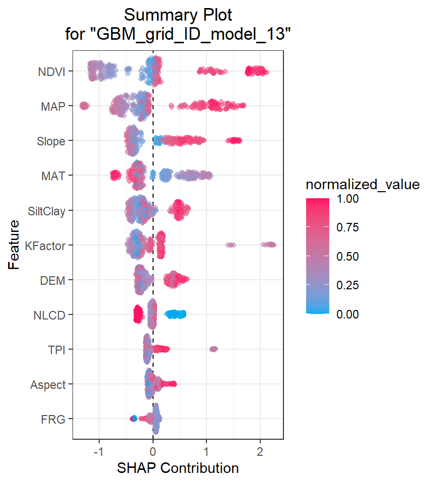
A partial dependence plot (PDP) is a graphical tool for understanding the relationship between a particular input feature and the output of a machine learning model.
A PDP shows the marginal effect of a single feature on the predicted outcome while holding all other features at a fixed value or their average value. The PDP can help to visualize the shape and direction of the relationship between the feature and the output, and can also help to identify any non-linearities or interactions between the feature and other features in the model.
To create a PDP, the value of the feature of interest is varied over its range, and the model’s predicted output is recorded for each value. The resulting data is then plotted on a graph, with the feature’s value on the x-axis and the predicted output on the y-axis.
PDPs can be used to gain insights into how a model is making its predictions and to identify which features are most important for the model’s output. They can also be used to identify potential biases in the model or to detect interactions between features that may be difficult to detect using other methods.
h2o.pd_multi_plot(best_GBM, h_train, "NDVI")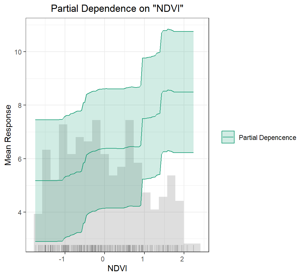
Residual Analysis plots the fitted values vs residuals on a test dataset. Ideally, residuals should be randomly distributed. Patterns in this plot can indicate potential problems with the model selection, e.g., using simpler model than necessary, not accounting for heteroscedasticity, autocorrelation, etc. Note that if you see “striped” lines of residuals, that is an artifact of having an integer valued (vs a real valued) response variable
h2o.residual_analysis_plot(best_GBM, h_train)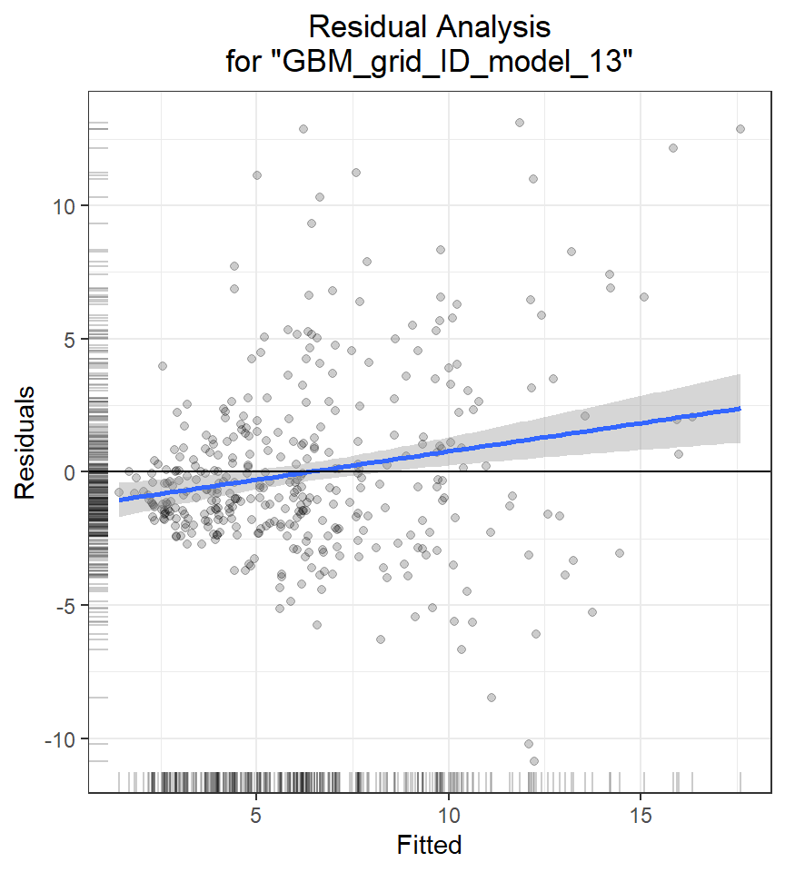
#  remove all object
rm(list = ls())Create a R-Markdown documents (name homework_14.rmd) in this project and do all Tasks using the data shown below.
Submit all codes and output as a HTML document (homework_14.html) before class of next week.
tidyverse, caret, Metrics, tidymodels, vip
Download the data and save in your project directory. Use read_csv to load the data in your R-session. For example:
mf<-read_csv(“bd_soil_update.csv”)
Create a data-frame with following variables for Rajshahi Division:
First use filter() to select data from Rajshai division and then use select() functions to create data-frame with following variables:
SOM, DEM, NDVI, NDFI,
Fit and show the model performance of a GBM model with using GBM packages.
Find the best GBM model with grid search using h2o and show all steps as shown in the tutorials,
Source: StatQuest with Josh Starme