Deep Neural Network with Keras-Tensorflow

Keras is a popular high-level deep learning library that provides a convenient and user-friendly API for building and training deep learning models. TensorFlow is a powerful open-source deep learning framework that serves as the backend for Keras and provides efficient computation for training and running deep learning models.

While Keras is primarily known for its Python implementation, it also has support for other programming languages, including R. In R, you can use the keras package which provides an interface to the Keras library with TensorFlow

Installation

To install TensorFlow in R, you can use the reticulate package, which provides an interface to Python from within R. Prior to using the tensorflow R package you need to install a version of Python and TensorFlow on your system. Below we describe how to install to do this as well the various options available for customizing your installation. Please follow instruction describe here.

First configure R with a Python installation it can use, like this:

library(reticulate)

path_to_python <- install_python()

virtualenv_create(“r-reticulate”, python = path_to_python)

Then use install_keras(), which installes Tensorflow, in addition to some commonly used packages like “scipy” and “tensorflow-datasets”.

install.packages(“keras”)

library(keras)

install_keras(envname = “r-reticulate”)

You can confirm that the installation succeeded with:

library(tensorflow)

tf$constant(“Hello Tensorflow!”)

Load Library

Code

library(tidyverse)
library(tidymodels)
library(tensorflow)
library(keras)
use_virtualenv("r-reticulate")

Data

In this exercise we will use following synthetic data set and will use DEM, Slope, TPI, MAT, MAP, NDVI, NLCD, and FRG variables to fit Deep Neural Network regression model. This data was created with AI using gp_soil_data data set

gp_soil_data_syn.csv

Code

# define file from my github
urlfile = "https://github.com//zia207/r-colab/raw/main/Data/USA/gp_soil_data_syn.csv"
mf<-read_csv(url(urlfile))
# Create a data-frame
df<-mf %>% dplyr::select(SOC, DEM, Slope, TPI,MAT, MAP,NDVI, NLCD, FRG)%>%
    glimpse()

Rows: 1,408
Columns: 9
$ SOC   <dbl> 1.900, 2.644, 0.800, 0.736, 15.641, 8.818, 3.782, 6.641, 4.803, …
$ DEM   <dbl> 2825.1111, 2535.1086, 1716.3300, 1649.8933, 2675.3113, 2581.4839…
$ Slope <dbl> 18.981682, 14.182393, 1.585145, 9.399726, 12.569353, 6.358553, 1…
$ TPI   <dbl> -0.91606224, -0.15259802, -0.39078590, -2.54008722, 7.40076303, …
$ MAT   <dbl> 4.709227, 4.648000, 6.360833, 10.265385, 2.798550, 6.358550, 7.0…
$ MAP   <dbl> 613.6979, 597.7912, 201.5091, 298.2608, 827.4680, 679.1392, 508.…
$ NDVI  <dbl> 0.6845260, 0.7557631, 0.2215059, 0.2785148, 0.7337426, 0.7017139…
$ NLCD  <chr> "Forest", "Forest", "Shrubland", "Shrubland", "Forest", "Forest"…
$ FRG   <chr> "Fire Regime Group IV", "Fire Regime Group IV", "Fire Regime Gro…

Inspect the data

Review the joint distribution of a few pairs of columns from the training set using GGally package.

Code

df_01<-df %>% dplyr::select(SOC, DEM, Slope,  TPI, MAT, MAP,NDVI )%>%
    glimpse()

Rows: 1,408
Columns: 7
$ SOC   <dbl> 1.900, 2.644, 0.800, 0.736, 15.641, 8.818, 3.782, 6.641, 4.803, …
$ DEM   <dbl> 2825.1111, 2535.1086, 1716.3300, 1649.8933, 2675.3113, 2581.4839…
$ Slope <dbl> 18.981682, 14.182393, 1.585145, 9.399726, 12.569353, 6.358553, 1…
$ TPI   <dbl> -0.91606224, -0.15259802, -0.39078590, -2.54008722, 7.40076303, …
$ MAT   <dbl> 4.709227, 4.648000, 6.360833, 10.265385, 2.798550, 6.358550, 7.0…
$ MAP   <dbl> 613.6979, 597.7912, 201.5091, 298.2608, 827.4680, 679.1392, 508.…
$ NDVI  <dbl> 0.6845260, 0.7557631, 0.2215059, 0.2785148, 0.7337426, 0.7017139…

Data Pre-processing

Code

dataset <- recipe(SOC ~ ., data = df) %>%
  step_zv(all_predictors()) %>%
  step_dummy(all_nominal()) %>%
  prep() %>%
  bake(new_data = NULL) %>%
  glimpse()

Rows: 1,408
Columns: 15
$ DEM                       <dbl> 2825.1111, 2535.1086, 1716.3300, 1649.8933, …
$ Slope                     <dbl> 18.981682, 14.182393, 1.585145, 9.399726, 12…
$ TPI                       <dbl> -0.91606224, -0.15259802, -0.39078590, -2.54…
$ MAT                       <dbl> 4.709227, 4.648000, 6.360833, 10.265385, 2.7…
$ MAP                       <dbl> 613.6979, 597.7912, 201.5091, 298.2608, 827.…
$ NDVI                      <dbl> 0.6845260, 0.7557631, 0.2215059, 0.2785148, …
$ SOC                       <dbl> 1.900, 2.644, 0.800, 0.736, 15.641, 8.818, 3…
$ NLCD_Herbaceous           <dbl> 0, 0, 0, 0, 0, 0, 0, 0, 0, 0, 0, 0, 1, 1, 0,…
$ NLCD_Planted.Cultivated   <dbl> 0, 0, 0, 0, 0, 0, 0, 0, 0, 0, 0, 0, 0, 0, 0,…
$ NLCD_Shrubland            <dbl> 0, 0, 1, 1, 0, 0, 0, 0, 0, 0, 0, 0, 0, 0, 0,…
$ FRG_Fire.Regime.Group.II  <dbl> 0, 0, 0, 0, 0, 0, 0, 0, 0, 0, 0, 0, 1, 0, 0,…
$ FRG_Fire.Regime.Group.III <dbl> 0, 0, 0, 0, 0, 0, 0, 1, 1, 1, 0, 0, 0, 1, 0,…
$ FRG_Fire.Regime.Group.IV  <dbl> 1, 1, 1, 0, 0, 0, 0, 0, 0, 0, 1, 1, 0, 0, 1,…
$ FRG_Fire.Regime.Group.V   <dbl> 0, 0, 0, 1, 1, 0, 0, 0, 0, 0, 0, 0, 0, 0, 0,…
$ FRG_Indeterminate.FRG     <dbl> 0, 0, 0, 0, 0, 0, 0, 0, 0, 0, 0, 0, 0, 0, 0,…

Split the data into training and test sets

Code

split <- initial_split(dataset, 0.8, strata = SOC)
train_dataset <- training(split)
test_dataset <- testing(split)

Split features from labels (SOC)

Separate the target or response value—the “label” (SOC) from the features. This label is the value that you will train the model to predict.

Code

train_features <- train_dataset %>% select(-SOC)
test_features <- test_dataset %>% select(-SOC)

train_labels <- train_dataset %>% select(SOC)
test_labels <- test_dataset %>% select(SOC)

Data Normalization

It is good practice to normalize features that use different scales and ranges.

One reason this is important is because the features are multiplied by the model weights. So, the scale of the outputs and the scale of the gradients are affected by the scale of the inputs.

Although a model might converge without feature normalization, normalization makes training much more stable.

Note: There is no advantage to normalizing the one-hot features—it is done here for simplicity. For more details on how to use the preprocessing layers, refer to the Working with preprocessing layers guide and the Classify structured data using Keras preprocessing layers tutorial.

Source:(https://tensorflow.rstudio.com/tutorials/keras/regression#inspect-the-data

The Normalization layer

The layer_normalization() is a clean and simple way to add feature normalization into your model.

The first step is to create the layer:

Code

normalizer <- layer_normalization(axis = -1L)

Then, fit the state of the preprocessing layer to the data by calling adapt():

Code

normalizer %>% adapt(as.matrix(train_features))

Duild and Complie Model

The normalization layer for a multiple-input model).
Two hidden, non-linear, Dense layers with the ReLU (relu) activation function nonlinearity.
A linear Dense single-output layer.

Both models will use the same training procedure so the compile method is included in the build_and_compile_model function below.

Code

build_and_compile_model <- function(norm) {
  model <- keras_model_sequential() %>%
    norm() %>%
    layer_dense(64, activation = 'relu') %>%
    layer_dense(64, activation = 'relu') %>%
    layer_dense(1)

  model %>% compile(
    loss = 'mean_absolute_error',
    optimizer = optimizer_adam(0.001)
  )

  model
}

Code

dnn_model <- build_and_compile_model(normalizer)
summary(dnn_model)

Model: "sequential"
________________________________________________________________________________
 Layer (type)                  Output Shape               Param #    Trainable  
================================================================================
 normalization (Normalization)  (None, 14)                29         Y          
 dense_2 (Dense)               (None, 64)                 960        Y          
 dense_1 (Dense)               (None, 64)                 4160       Y          
 dense (Dense)                 (None, 1)                  65         Y          
================================================================================
Total params: 5,214
Trainable params: 5,185
Non-trainable params: 29
________________________________________________________________________________

Use Keras fit() to execute the training for 100 epochs:

Code

history <- dnn_model %>% fit(
  as.matrix(train_features),
  as.matrix(train_labels),
  validation_split = 0.1,
  verbose = 0,
  epochs = 100
)

Code

plot(history)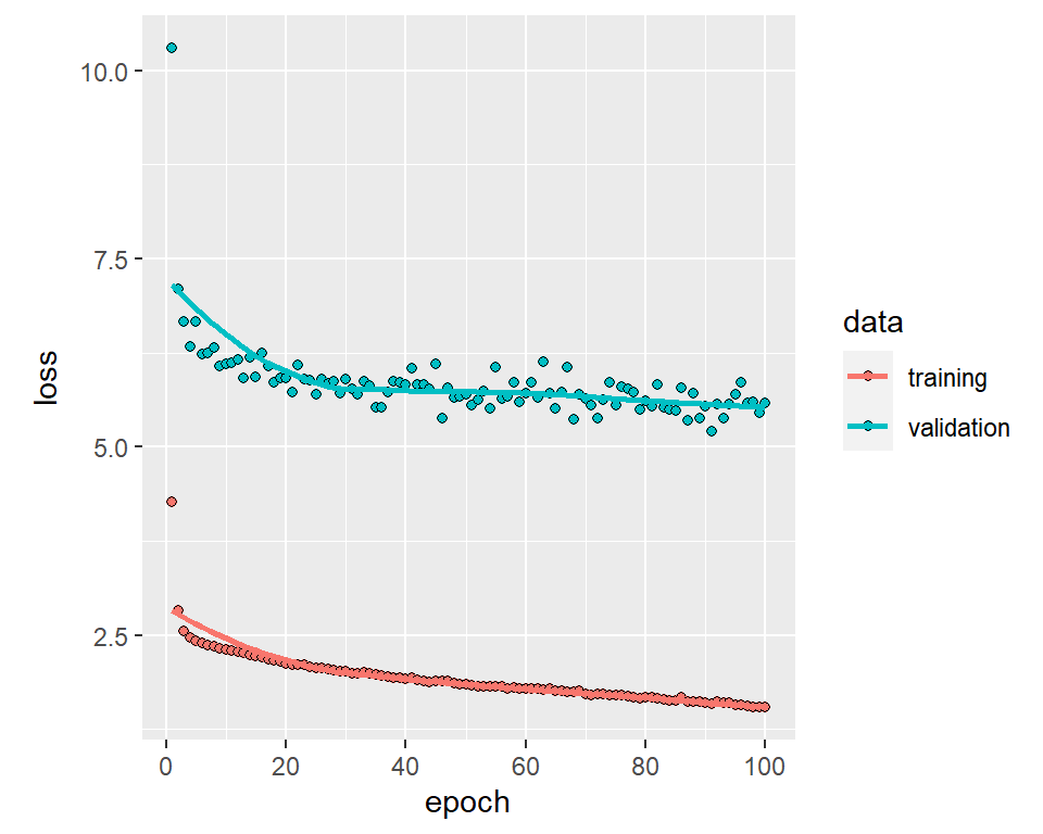

Prediction

Code

test_results <- list()

test_results[['dnn_model']] <- dnn_model %>% evaluate(
  as.matrix(test_features),
  as.matrix(test_labels),
  verbose = 0
)

Code

test_results

$dnn_model
    loss 
2.076994

Code

test_labels$Pred.SOC <- as.data.frame(predict(dnn_model, as.matrix(test_features)))

Code

names(test_labels)

[1] "SOC"      "Pred.SOC"

Code

RMSE<- Metrics::rmse(test_labels$SOC, test_labels$Pred.SOC$V1)
MAE<- Metrics::mae(test_labels$SOC, test_labels$Pred.SOC$V1)

# Print results
paste0("RMSE: ", round(RMSE,2))

[1] "RMSE: 3.5"

Code

paste0("MAE: ", round(MAE,2))

[1] "MAE: 2.08"

Code

library(ggpmisc)
formula<-y~x

ggplot(test_labels, aes(SOC,Pred.SOC$V1)) +
  geom_point() +
  geom_smooth(method = "lm")+
  stat_poly_eq(use_label(c("eq", "adj.R2")), formula = formula) +
  ggtitle("DNN-Keras") +
  xlab("Observed") + ylab("Predicted") +
  scale_x_continuous(limits=c(0,25), breaks=seq(0, 25, 5))+ 
  scale_y_continuous(limits=c(0,25), breaks=seq(0, 25, 5)) +
  # Flip the bars
  theme(
    panel.background = element_rect(fill = "grey95",colour = "gray75",size = 0.5, linetype = "solid"),
    axis.line = element_line(colour = "grey"),
    plot.title = element_text(size = 14, hjust = 0.5),
    axis.title.x = element_text(size = 14),
    axis.title.y = element_text(size = 14),
    axis.text.x=element_text(size=13, colour="black"),
    axis.text.y=element_text(size=13,angle = 90,vjust = 0.5, hjust=0.5, colour='black'))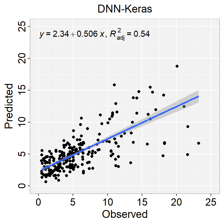

Code

#  remove all object
rm(list = ls())

Tuning Keras-DNN with Tidymodel

Load Library

Code

library(tidyverse)
library(tidymodels)
library(tensorflow)
library(keras)
use_virtualenv("r-reticulate")

Data

gp_soil_data_syn.csv

Code

# define file from my github
urlfile = "https://github.com//zia207/r-colab/raw/main/Data/USA/gp_soil_data_syn.csv"
mf<-read_csv(url(urlfile))
# Create a data-frame
df<-mf %>% dplyr::select(SOC, DEM, Slope, TPI,MAT, MAP,NDVI, NLCD, FRG)%>%
    glimpse()

Rows: 1,408
Columns: 9
$ SOC   <dbl> 1.900, 2.644, 0.800, 0.736, 15.641, 8.818, 3.782, 6.641, 4.803, …
$ DEM   <dbl> 2825.1111, 2535.1086, 1716.3300, 1649.8933, 2675.3113, 2581.4839…
$ Slope <dbl> 18.981682, 14.182393, 1.585145, 9.399726, 12.569353, 6.358553, 1…
$ TPI   <dbl> -0.91606224, -0.15259802, -0.39078590, -2.54008722, 7.40076303, …
$ MAT   <dbl> 4.709227, 4.648000, 6.360833, 10.265385, 2.798550, 6.358550, 7.0…
$ MAP   <dbl> 613.6979, 597.7912, 201.5091, 298.2608, 827.4680, 679.1392, 508.…
$ NDVI  <dbl> 0.6845260, 0.7557631, 0.2215059, 0.2785148, 0.7337426, 0.7017139…
$ NLCD  <chr> "Forest", "Forest", "Shrubland", "Shrubland", "Forest", "Forest"…
$ FRG   <chr> "Fire Regime Group IV", "Fire Regime Group IV", "Fire Regime Gro…

Data split

The data set (n = 1408) will randomly split into sub-sets for training (70%), validation (15%) and test data (15%). The validation data will be used to optimized the model parameters during the tuning and training processes. The test data set will be used as the hold-out data to evaluate the DNN model.

Code

set.seed(1245)   # for reproducibility
library(tidymodels)
split <- initial_split(df, prop = 0.8, strata = SOC)
train <- split %>% training()
test <-  split %>% testing()

Data Pre-processing

Code

dnn_recipe <-
  recipe(SOC ~ ., data = train) %>%
  step_zv(all_predictors()) %>%
  step_dummy(all_nominal()) %>%
  step_normalize(all_numeric_predictors())

# For testing when we arrive at a final model: 
test_normalized <- bake(prep(dnn_recipe), new_data = test, all_predictors())

# Set 10 fold cross-validation data set 
cv_folds<- vfold_cv(train, v=5)

Specify tunable Hypermeters of Keras - DNN

Code

dnn_model <- 
  mlp(mode = "regression", 
      hidden_units = tune(),
      dropout = tune(),
      epochs = tune(),
      activation = "relu",
      ) %>%
      set_engine("keras", 
                 verbose = 0,
                 optimizer = optimizer_adam(0.001),
                 validation = .10)

dnn_model

Single Layer Neural Network Model Specification (regression)

Main Arguments:
  hidden_units = tune()
  dropout = tune()
  epochs = tune()
  activation = relu

Engine-Specific Arguments:
  verbose = 0
  optimizer = optimizer_adam(0.001)
  validation = 0.1

Computational engine: keras

Create Workflow

Code

dnn_wf <- workflow() %>% 
    add_model(dnn_model) %>% 
    add_recipe(dnn_recipe)

dnn_wf

══ Workflow ════════════════════════════════════════════════════════════════════
Preprocessor: Recipe
Model: mlp()

── Preprocessor ────────────────────────────────────────────────────────────────
3 Recipe Steps

• step_zv()
• step_dummy()
• step_normalize()

── Model ───────────────────────────────────────────────────────────────────────
Single Layer Neural Network Model Specification (regression)

Main Arguments:
  hidden_units = tune()
  dropout = tune()
  epochs = tune()
  activation = relu

Engine-Specific Arguments:
  verbose = 0
  optimizer = optimizer_adam(0.001)
  validation = 0.1

Computational engine: keras

Define random grid prameters

Code

dnn_grid <- parameters(dnn_model) %>% 
    finalize(train) %>% 
    grid_random(size = 10)
head(dnn_grid)

# A tibble: 6 × 3
  hidden_units  dropout epochs
         <int>    <dbl>  <int>
1            1 0.000795    125
2           10 0.515       557
3            9 0.414       345
4            5 0.0478      811
5            2 0.896        20
6            2 0.635       684

Tune Grid

Code

#doParallel::registerDoParallel()

set.seed(345)
# grid search
dnn_tune_grid <- dnn_wf %>%
    tune_grid(
        resamples = cv_folds,
        grid = dnn_grid,
        control = control_grid(verbose = F),
        metrics = metric_set(rmse, rsq, mae)
    )

Code

collect_metrics(dnn_tune_grid )

# A tibble: 30 × 9
   hidden_units  dropout epochs .metric .estimator  mean     n std_err .config  
          <int>    <dbl>  <int> <chr>   <chr>      <dbl> <int>   <dbl> <chr>    
 1            1 0.000795    125 mae     standard   3.59      5 0.253   Preproce…
 2            1 0.000795    125 rmse    standard   5.49      5 0.461   Preproce…
 3            1 0.000795    125 rsq     standard   0.182     2 0.170   Preproce…
 4           10 0.515       557 mae     standard   2.84      5 0.0727  Preproce…
 5           10 0.515       557 rmse    standard   4.06      5 0.151   Preproce…
 6           10 0.515       557 rsq     standard   0.353     5 0.00975 Preproce…
 7            9 0.414       345 mae     standard   2.75      5 0.103   Preproce…
 8            9 0.414       345 rmse    standard   3.92      5 0.181   Preproce…
 9            9 0.414       345 rsq     standard   0.401     5 0.0208  Preproce…
10            5 0.0478      811 mae     standard   2.76      5 0.129   Preproce…
# ℹ 20 more rows

Code

autoplot(dnn_tune_grid)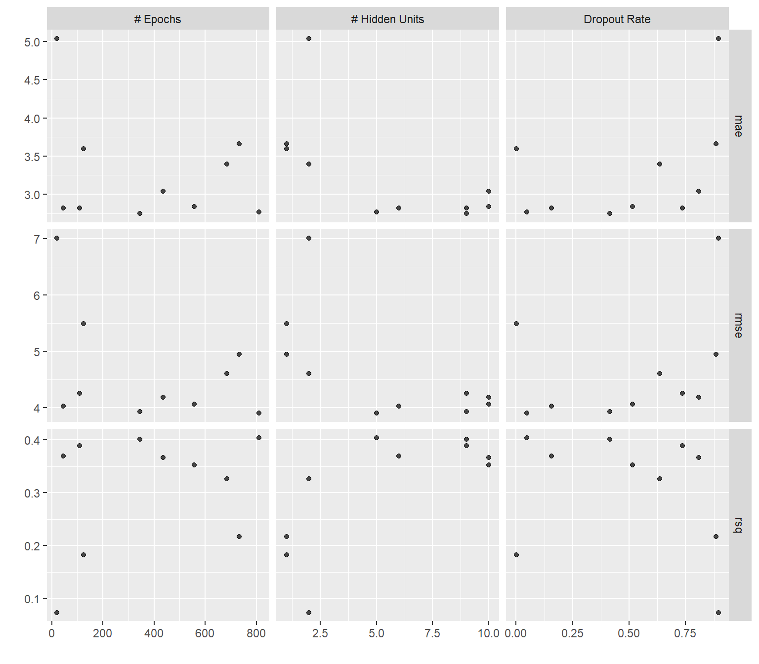

The best DNN model

Code

best_rmse <- select_best(dnn_tune_grid , "rmse")

dnn_final <- finalize_model(
  dnn_model,
  best_rmse
)

dnn_final

Single Layer Neural Network Model Specification (regression)

Main Arguments:
  hidden_units = 5
  dropout = 0.0477566176559776
  epochs = 811
  activation = relu

Engine-Specific Arguments:
  verbose = 0
  optimizer = optimizer_adam(0.001)
  validation = 0.1

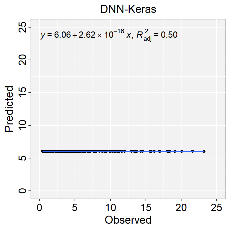
Computational engine: keras

Fit the model

Code

final_fit <- fit(dnn_final, SOC ~ ., data = train)

Prediction

Code

test$SOC.pred = predict(final_fit, test)

Code

library(Metrics)
RMSE<- Metrics::rmse(test$SOC, test$SOC.pred$.pred)
RMSE

[1] 4.933049

Code

library(ggpmisc)
formula<-y~x

ggplot(test, aes(SOC,SOC.pred$.pred)) +
  geom_point() +
  geom_smooth(method = "lm")+
  stat_poly_eq(use_label(c("eq", "adj.R2")), formula = formula) +
  ggtitle("DNN-Keras") +
  xlab("Observed") + ylab("Predicted") +
  scale_x_continuous(limits=c(0,25), breaks=seq(0, 25, 5))+ 
  scale_y_continuous(limits=c(0,25), breaks=seq(0, 25, 5)) +
  # Flip the bars
  theme(
    panel.background = element_rect(fill = "grey95",colour = "gray75",size = 0.5, linetype = "solid"),
    axis.line = element_line(colour = "grey"),
    plot.title = element_text(size = 14, hjust = 0.5),
    axis.title.x = element_text(size = 14),
    axis.title.y = element_text(size = 14),
    axis.text.x=element_text(size=13, colour="black"),
    axis.text.y=element_text(size=13,angle = 90,vjust = 0.5, hjust=0.5, colour='black'))

Deep Neural Network with Keras-Tensorflow

Installation

Load Library

Data

Inspect the data

Data Pre-processing

Split the data into training and test sets

Split features from labels (SOC)

Data Normalization

The Normalization layer

Duild and Complie Model

Prediction

Tuning Keras-DNN with Tidymodel

Load Library

Data

Data split

Data Pre-processing

Specify tunable Hypermeters of Keras - DNN

Create Workflow

Define random grid prameters

Tune Grid

The best DNN model

Fit the model

Prediction

Further Reading