Regularized Generalized Linear Models (GLMs) are a family of statistical models that combine the benefits of generalized linear models (GLMs) with regularization techniques to improve generalization performance and reduce overfitting. Overfitting occurs when a model becomes too complex and starts fitting the noise in the data, resulting in poor performance on new, unseen data. Regularization addresses this issue by adding a penalty term to the loss function that the model is trying to minimize.
Several regularization techniques include L1 regularization (Lasso), L2 regularization (Ridge), and Elastic Net regularization. Like classical linear regression, Ridge and Lasso also build the linear model, but their fundamental peculiarity is regularization. These methods aim to improve the loss function so that it depends on the sum of the squared differences and the regression coefficients.
L1 regularization adds a penalty term proportional to the absolute value of the coefficients, which results in sparse solutions where some coefficients are precisely zero. This can be used for feature selection, as it tends to set coefficients of less important features to zero.
L2 regularization adds a penalty term proportional to the square of the coefficients, which tends to shrink the coefficients towards zero, but does not set them precisely to zero. This can be useful when all the features are necessary, but some may have minimal effects.
Elastic Net regularization combines L1 and L2 regularization and balances feature selection and coefficient shrinkage.
Regularization can be a powerful tool for improving the performance of machine learning models, mainly when dealing with high-dimensional data or datasets with a limited number of observations. It can help to prevent overfitting, improve the interpretability of the model, and provide insights into the importance of different features in the data.
Note
In machine learning, a loss function is a mathematical function that measures the difference between the predicted output of a model and the actual output given a set of input data. The loss function quantifies how well the model performs and provides a way to optimize the model’s parameters during training.
The goal of machine learning is to minimize the loss function, which represents the error between the predicted output of the model and the actual output. By minimizing the loss function, the model learns to make better predictions on new data that it has not seen before.
Ridge, Lasso, and Elastic Net Regressions
Lasso and Ridge and regression is a linear regression technique that adds an L1 and L2 regularization term to the cost function to prevent overfitting, respectively. The regularization term adds a penalty to the sum of squared regression coefficients, which shrinks the coefficients toward zero. The regularization parameter, alpha, controls the strength of the regularization. Larger alpha values result in more shrinkage of the coefficients towards zero and can lead to a simpler model with reduced variance but potentially increased bias. Smaller values of alpha result in less shrinkage and a model that is closer to ordinary linear regression.
Ridge and Lasso regressions can be used when there is multicollinearity among the predictor variables, which can cause instability in the estimates of the regression coefficients. By adding the regularization term, ridge regression can help stabilize the estimates and improve the model’s accuracy.
Elastic Net regularization is a combination of Lasso and Ridge regularization techniques. Elastic Net regularization adds two penalty terms to the cost function of a linear regression model: the L1 penalty and the L2 penalty. The L1 penalty encourages sparsity in the model by setting some of the coefficients to zero, while the L2 penalty shrinks the magnitude of the coefficients toward zero.
The Elastic Net penalty term is a weighted sum of the L1 and L2 penalties, controlled by a hyperparameter called alpha. When alpha is set to zero, Elastic Net is equivalent to Ridge regularization, and when alpha is set to one, Elastic Net is equivalent to Lasso regularization.
The “glmnet” method in caret has an alpha argument that determines what type of model is fit. If alpha = 0 then a ridge regression model is fit; if alpha = 1 then a lasso model is fi, a a value between 0 and 1 (say 0.3) for elastic net regression will be fit. Here we’ll use caret as a wrapper for glment package.
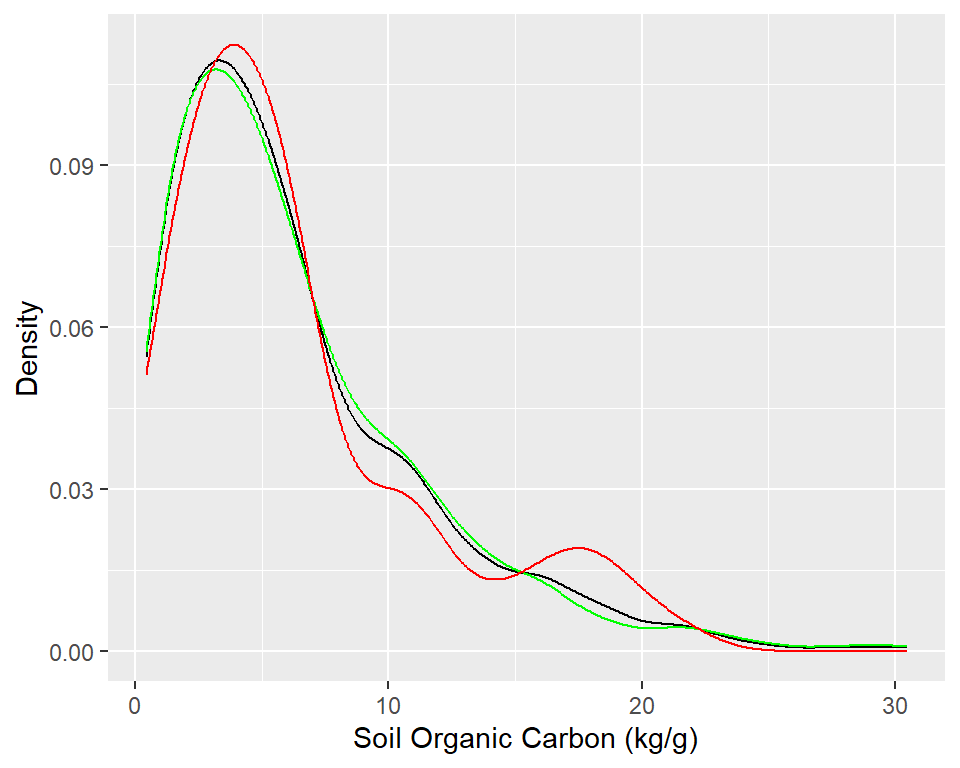
The function createDataPartition of caret package can be used to create balanced splits of the data
Code
set.seed(3456)trainIndex <-createDataPartition(dummies.df$SOC, p = .80, list =FALSE, times =1)df_train <- dummies.df[ trainIndex,]df_test <- dummies.df[-trainIndex,]
Code
# Density plot all, train and test data ggplot()+geom_density(data = dummies.df, aes(SOC))+geom_density(data = df_train, aes(SOC), color ="green")+geom_density(data = df_test, aes(SOC), color ="red") +xlab("Soil Organic Carbon (kg/g)") +ylab("Density")
Set control prameters
Code
set.seed(123)train.control <-trainControl(method ="repeatedcv", number =10, repeats =5,preProc =c("center", "scale", "nzv"))
glmnet

375 samples
 19 predictor

No pre-processing
Resampling: Cross-Validated (10 fold, repeated 5 times)
Summary of sample sizes: 338, 336, 337, 338, 338, 337, ...
Resampling results:

  RMSE      Rsquared   MAE
  4.109635  0.3864478  3.004719

Tuning parameter 'alpha' was held constant at a value of 1
Tuning
 parameter 'lambda' was held constant at a value of 1
Code
print(model.ridge)
glmnet

375 samples
 19 predictor

No pre-processing
Resampling: Cross-Validated (10 fold, repeated 5 times)
Summary of sample sizes: 337, 338, 339, 335, 338, 339, ...
Resampling results:

  RMSE      Rsquared   MAE
  3.872206  0.4199461  2.792984

Tuning parameter 'alpha' was held constant at a value of 0
Tuning
 parameter 'lambda' was held constant at a value of 1
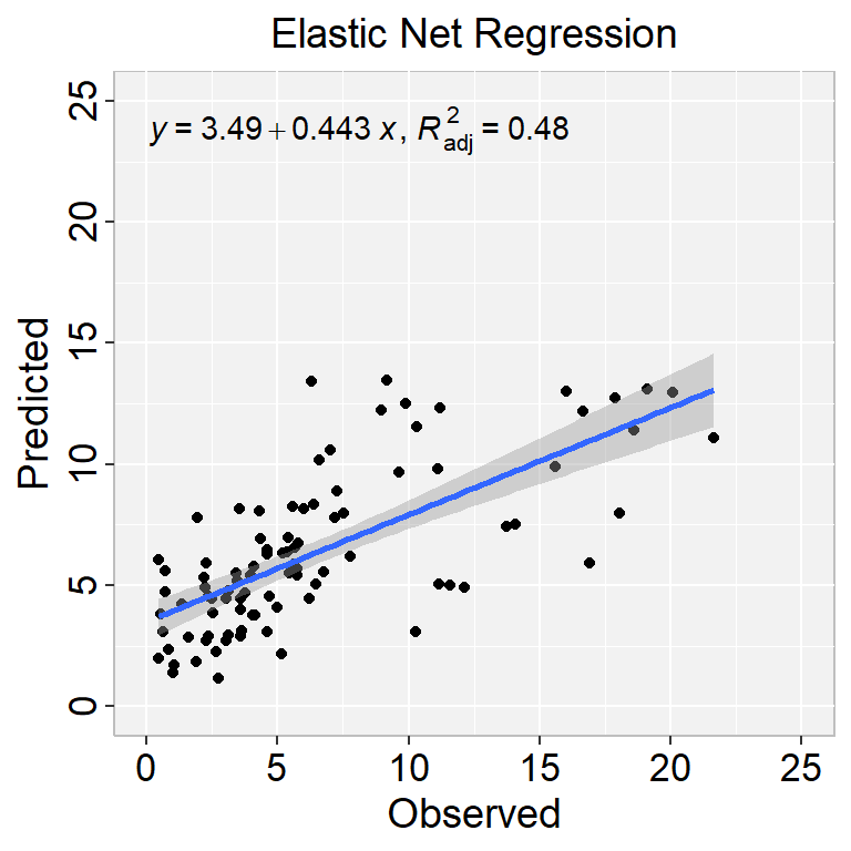
The elastic net regression can be easily computed using the caret workflow, with glmnet package. We use caret to automatically select the best tuning parameters alpha and lambda. The caret packages tests a range of possible alpha and lambda values, then selects the best values for lambda and alpha, resulting to a final model that is an elastic net model.
Here, we’ll test the combination of 10 different values for alpha and lambda. This is specified using the option tuneLength. The best alpha and lambda values are those values that minimize the cross-validation error.
Code
# Elastic Net Regressionmodel.elasticNet <-train(SOC ~., data = df_train, method ="glmnet",trControl = train.control,tuneLength =10)
The tidymodels provides a comprehensive framework for building, tuning, and evaluating regularized GLM models in R while following the principles of the tidyverse.
install.packages(“tidymodels”)
Split Data
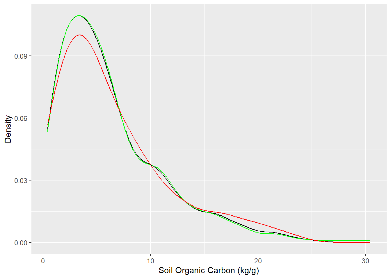
We use rsample package, install with tidymodels, to split data into training (70%) and test data (30%) set with Stratified Random Sampling. initial_split() creates a single binary split of the data into a training set and testing set.
Note
Stratified random sampling is a technique for selecting a representative sample from a population, where the sample is chosen in a way that ensures that certain subgroups within the population are adequately represented in the sample.
Code
##| fig.width: 4#| fig.height: 4library(tidymodels)set.seed(1245) # for reproducibilitysplit <-initial_split(df, prop =0.8, strata = SOC)train <- split %>%training()test <- split %>%testing()# Set 10 fold cross-validation data set cv_fold <-vfold_cv(train, v =10)# Density plot all, train and test data ggplot()+geom_density(data = df, aes(SOC))+geom_density(data = train, aes(SOC), color ="green")+geom_density(data = test, aes(SOC), color ="red") +xlab("Soil Organic Carbon (kg/g)") +ylab("Density")
Create Recipe
A recipe is a description of the steps to be applied to a data set in order to prepare it for data analysis. Before training the model, we can use a recipe to do some preprocessing required by the model.
Code
# load librarylibrary(tidymodels)# Create a recipemodel_recipe <-recipe(SOC ~ ., data = train) %>%step_zv(all_predictors()) %>%step_dummy(all_nominal()) %>%step_normalize(all_numeric_predictors())
Build a Ridge Regression model
set_engine() is used to specify which package or system will be used to fit the model, along with any arguments specific to that software. We will use “glm” without any regularization parameters. The mixture argument specifies the amount of different types of regularization, mixture = 0 specifies only ridge regularization and mixture = 1 specifies only lasso regularization. When using the glmnet engine, we also need to set a penalty to be able to fit the model. The penalty = tune() tells tune_grid() that penalty parameter should be tuned.
A workflow is a container object that aggregates information required to fit and predict from a model. This information might be a recipe used in pre-processing, specified through add_recipe(), or the model specification to fit, specified through add_model().
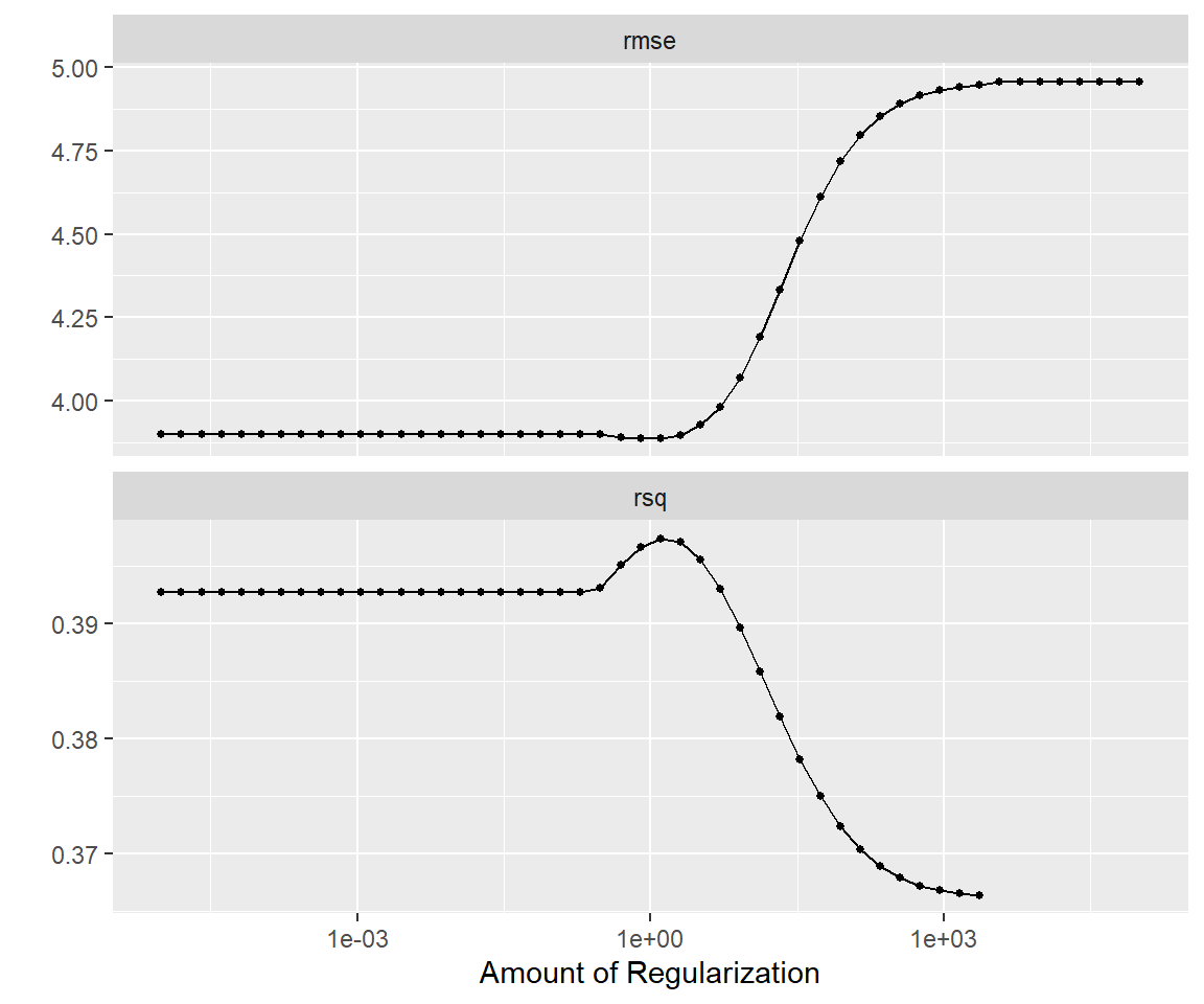
This can be created using grid_regular() which creates a grid of evenly spaces parameter values. We use the penalty() function from the dials package to denote the parameter and set the range of the grid we are searching for. Note that this range is log-scaled.
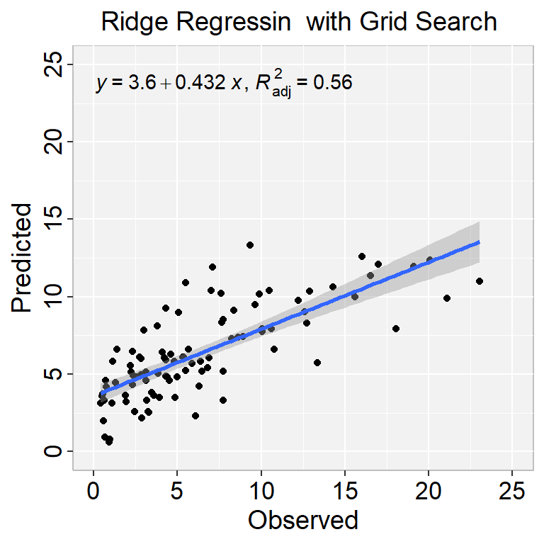
This value of penalty can then be used with finalize_workflow() to update/finalize the recipe by replacing tune() with the value of best_penalty. Now, this model should be fit again, this time using the whole training data set.
Code
# update penaltyridge_final <-finalize_workflow(ridge_wflow, best_penalty)# fit the modelridge_final_fit <-fit(ridge_final, data = train)
This object has the finalized recipe and fitted model objects inside. You may want to extract the model or recipe objects from the workflow. To do this, you can use the helper functions extract_fit_parsnip():
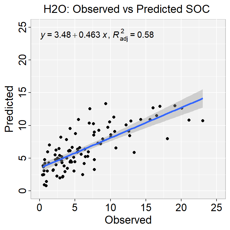
The h2o package provides an open-source implementation of GLM that is specifically designed for big data. To use the GLM function in h2o, you will need to first install and load the package in your R environment.
H2O supports elastic net regularization, which is a combination of the l1 and l2 penalties parametrized by the alpha and lambda arguments.
alpha controls the elastic net penalty distribution between the l1 and l2 norms. It can have any value in the [0; 1] range or a vector of values (which triggers grid search). If alpha = 0, H2O solves the GLM using ridge regression. If alpha = 1, the Lasso penalty is used.
lambda controls the penalty strength. The range is any positive value or a vector of values (which triggers grid search).
We will use Random Grid Search (RGS) to find the optimal parameters for the GLM models. We employ the K-fold cross validation method to determine the optimal hyper-parameters from a set of all possible hyper-parameter value combinations of alpha and lambda.
We can view the results of the grid search by printing the grid object. We can use this information to select the best model based on its CV performance and then use it to make predictions on new data.
library(tidymodels)set.seed(1245) # for reproducibilitysplit.df <-initial_split(df, prop =0.8, strata = SOC)train.df <- split.df %>%training()test.df <- split.df %>%testing()# Set 10 fold cross-validation data set
Code
#| warning: false#| error: falselibrary(h2o)
----------------------------------------------------------------------

Your next step is to start H2O:
    > h2o.init()

For H2O package documentation, ask for help:
    > ??h2o

After starting H2O, you can use the Web UI at http://localhost:54321
For more information visit https://docs.h2o.ai

----------------------------------------------------------------------
Attaching package: 'h2o'
The following objects are masked from 'package:lubridate':

    day, hour, month, week, year
The following objects are masked from 'package:stats':

    cor, sd, var
The following objects are masked from 'package:base':

    %*%, %in%, &&, ||, apply, as.factor, as.numeric, colnames,
    colnames<-, ifelse, is.character, is.factor, is.numeric, log,
    log10, log1p, log2, round, signif, trunc
H2O is not running yet, starting it now...

Note:  In case of errors look at the following log files:
    C:\Users\zahmed2\AppData\Local\Temp\1\RtmpEdicW7\file34081f6eefe/h2o_zahmed2_started_from_r.out
    C:\Users\zahmed2\AppData\Local\Temp\1\RtmpEdicW7\file340818436689/h2o_zahmed2_started_from_r.err


Starting H2O JVM and connecting:  Connection successful!

R is connected to the H2O cluster:
    H2O cluster uptime:         3 seconds 205 milliseconds
    H2O cluster timezone:       America/New_York
    H2O data parsing timezone:  UTC
    H2O cluster version:        3.40.0.4
    H2O cluster version age:    3 months and 23 days
    H2O cluster name:           H2O_started_from_R_zahmed2_qtu738
    H2O cluster total nodes:    1
    H2O cluster total memory:   148.00 GB
    H2O cluster total cores:    40
    H2O cluster allowed cores:  40
    H2O cluster healthy:        TRUE
    H2O Connection ip:          localhost
    H2O Connection port:        54321
    H2O Connection proxy:       NA
    H2O Internal Security:      FALSE
    R Version:                  R version 4.3.1 (2023-06-16 ucrt)
Warning in h2o.clusterInfo():
Your H2O cluster version is (3 months and 23 days) old. There may be a newer version available.
Please download and install the latest version from: https://h2o-release.s3.amazonaws.com/h2o/latest_stable.html
Code
#disable progress bar for RMarkdownh2o.no_progress() # Optional: remove anything from previous sessionh2o.removeAll()
We must find the optimal values of the alpha and lambda regularization parameters to get the best possible model. To find the optimal values, H2O provides grid search over alpha and lambda and a particular form of grid search called “lambda search” over lambda. For a detailed explanation, refer to Regularization. The recommended way to find optimal regularization settings on H2O is to do a grid search over a few alpha values with an automatic lambda search for each alpha.
The alpha parameter controls the distribution between the l1 (Lasso) and l2 (Ridge regression) penalties. A value of 1.0 for alpha represents Lasso, and an alpha value of 0.0 produces ridge regression. The lambda parameter controls the amount of regularization applied. If lambda is 0.0, no regularization is applied and the alpha parameter is ignored. The default value for lambda is calculated by H2O using a heuristic based on the training data. If you let H2O calculate the value for lambda, you can see the chosen value in the model output.
To perform a hyperparameter grid search in h2o R, you can use the h2o.grid() function. This function takes a set of hyperparameters and their corresponding values, and trains and evaluates models with all possible combinations of those hyperparameters.
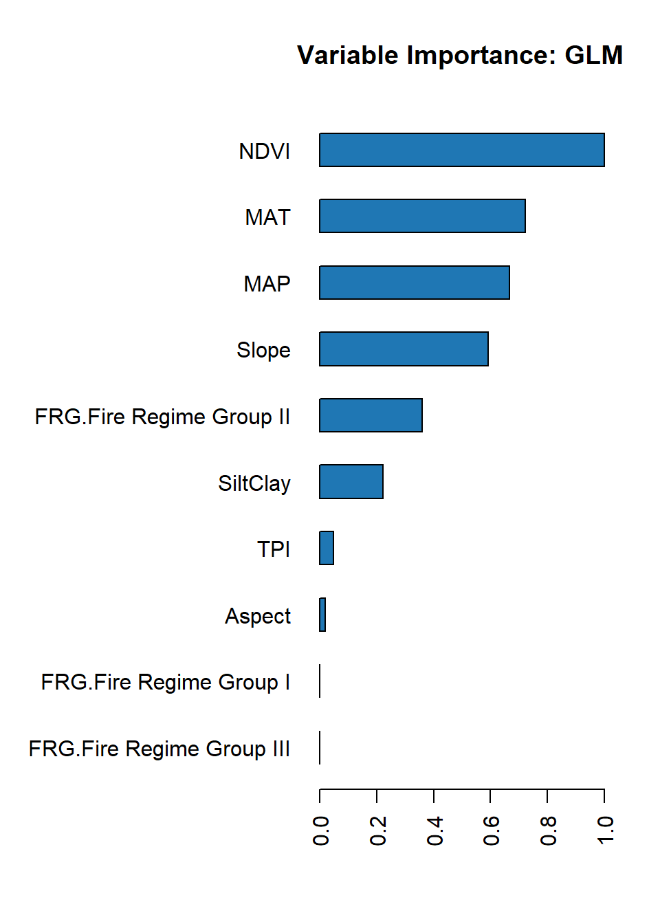
Variable importance in GLM regression model represents the coefficient magnitudes. The standardized coefficients are returned if the standardize option is enabled (which is the default). These are the predictor weights of the standardized data and are included only for informational purposes like comparing the relative variable importance.
Code
# Retrieve the variable importanceh2o.varimp(best_glm)
Variable Importances:
                    variable relative_importance scaled_importance percentage
1                       NDVI            1.428084          1.000000   0.275518
2                        MAT            1.032379          0.722912   0.199175
3                        MAP            0.953076          0.667381   0.183875
4                      Slope            0.844157          0.591111   0.162862
5   FRG.Fire Regime Group II            0.513842          0.359812   0.099135
6                   SiltClay            0.317600          0.222396   0.061274
7                        TPI            0.068080          0.047672   0.013135
8                     Aspect            0.026052          0.018243   0.005026
9    FRG.Fire Regime Group I            0.000000          0.000000   0.000000
10 FRG.Fire Regime Group III            0.000000          0.000000   0.000000
11  FRG.Fire Regime Group IV            0.000000          0.000000   0.000000
12   FRG.Fire Regime Group V            0.000000          0.000000   0.000000
13     FRG.Indeterminate FRG            0.000000          0.000000   0.000000
14               NLCD.Forest            0.000000          0.000000   0.000000
15           NLCD.Herbaceous            0.000000          0.000000   0.000000
16   NLCD.Planted/Cultivated            0.000000          0.000000   0.000000
17            NLCD.Shrubland            0.000000          0.000000   0.000000
18                       DEM            0.000000          0.000000   0.000000
19                   KFactor            0.000000          0.000000   0.000000
To plot variable importance for the model, we use the h2o.varimp_plot() function and pass the trained model as an argument. The function generates a bar plot of the relative importance of each input variable, sorted in descending order by importance.
The h2o.varimp_plot() function also has several optional arguments that you can use to customize the appearance of the plot, such as num_of_features to limit the number of features displayed on the plot, title to set a title for the plot, and col to set the color of the bars.
Code
h2o.varimp_plot(best_glm)
Exercise
Create a R-Markdown documents (name homework_12.rmd) in this project and do all Tasks using the data shown below.
Submit all codes and output as a HTML document (homework_12.html) before class of next week.
[{fig-align="right" width="176" height="64"}](https://github.com/zia207/r-colab/blob/main/regularized_glm.ipynb)# Regularized Generalized Linear Models {.unnumbered}Regularized Generalized Linear Models (GLMs) are a family of statistical models that combine the benefits of generalized linear models (GLMs) with regularization techniques to improve generalization performance and reduce overfitting. Overfitting occurs when a model becomes too complex and starts fitting the noise in the data, resulting in poor performance on new, unseen data. Regularization addresses this issue by adding a penalty term to the loss function that the model is trying to minimize.Several regularization techniques include L1 regularization (Lasso), L2 regularization (Ridge), and Elastic Net regularization. Like classical linear regression, Ridge and Lasso also build the linear model, but their fundamental peculiarity is regularization. These methods aim to improve the loss function so that it depends on the sum of the squared differences and the regression coefficients.L1 regularization adds a penalty term proportional to the absolute value of the coefficients, which results in sparse solutions where some coefficients are precisely zero. This can be used for feature selection, as it tends to set coefficients of less important features to zero.L2 regularization adds a penalty term proportional to the square of the coefficients, which tends to shrink the coefficients towards zero, but does not set them precisely to zero. This can be useful when all the features are necessary, but some may have minimal effects.Elastic Net regularization combines L1 and L2 regularization and balances feature selection and coefficient shrinkage.Regularization can be a powerful tool for improving the performance of machine learning models, mainly when dealing with high-dimensional data or datasets with a limited number of observations. It can help to prevent overfitting, improve the interpretability of the model, and provide insights into the importance of different features in the data.::: callout-noteIn machine learning, a loss function is a mathematical function that measures the difference between the predicted output of a model and the actual output given a set of input data. The loss function quantifies how well the model performs and provides a way to optimize the model's parameters during training.The goal of machine learning is to minimize the loss function, which represents the error between the predicted output of the model and the actual output. By minimizing the loss function, the model learns to make better predictions on new data that it has not seen before.:::### Ridge, Lasso, and Elastic Net RegressionsLasso and Ridge and regression is a linear regression technique that adds an L1 and L2 regularization term to the cost function to prevent overfitting, respectively. The regularization term adds a penalty to the sum of squared regression coefficients, which shrinks the coefficients toward zero. The regularization parameter, alpha, controls the strength of the regularization. Larger alpha values result in more shrinkage of the coefficients towards zero and can lead to a simpler model with reduced variance but potentially increased bias. Smaller values of alpha result in less shrinkage and a model that is closer to ordinary linear regression.Ridge and Lasso regressions can be used when there is multicollinearity among the predictor variables, which can cause instability in the estimates of the regression coefficients. By adding the regularization term, ridge regression can help stabilize the estimates and improve the model's accuracy.Elastic Net regularization is a combination of Lasso and Ridge regularization techniques. Elastic Net regularization adds two penalty terms to the cost function of a linear regression model: the L1 penalty and the L2 penalty. The L1 penalty encourages sparsity in the model by setting some of the coefficients to zero, while the L2 penalty shrinks the magnitude of the coefficients toward zero.The Elastic Net penalty term is a weighted sum of the L1 and L2 penalties, controlled by a hyperparameter called alpha. When alpha is set to zero, Elastic Net is equivalent to Ridge regularization, and when alpha is set to one, Elastic Net is equivalent to Lasso regularization.The "glmnet" method in caret has an alpha argument that determines what type of model is fit. If alpha = 0 then a ridge regression model is fit; if alpha = 1 then a lasso model is fi, a a value between 0 and 1 (say 0.3) for elastic net regression will be fit. Here we'll use caret as a wrapper for glment package.### DataIn this exercise we will use following data set.[gp_soil_data.csv](https://www.dropbox.com/s/9ikm5yct36oflei/gp_soil_data.csv?dl=0)```{r}#| warning: false#| error: false# define data folderdataFolder<-"E:/Dropbox/GitHub/Data/USA/"# Load Packageslibrary(tidyverse)# Load datamf<-read_csv(paste0(dataFolder, "gp_soil_data.csv"))# Create a data-framedf<-mf %>% dplyr::select(SOC, DEM, Slope, Aspect, TPI, KFactor, SiltClay, MAT, MAP,NDVI, NLCD, FRG)%>%glimpse()```## Ridge, Lasso, and Elastic Net Regressions with caret package### Create A Full Set of Dummy VariablesdummyVars() from caret package creates a full set of dummy variables (i.e. less than full rank parameterization)```{r}#| warning: false#| error: falselibrary(caret)# create dummy variabledummies <-dummyVars(SOC ~ ., data = df)dummies.df<-as.data.frame(predict(dummies, newdata = df))dummies.df$SOC<-df$SOC```### Data SplittingThe function createDataPartition of caret package can be used to create balanced splits of the data```{r}#| warning: false#| error: falseset.seed(3456)trainIndex <-createDataPartition(dummies.df$SOC, p = .80, list =FALSE, times =1)df_train <- dummies.df[ trainIndex,]df_test <- dummies.df[-trainIndex,]``````{r}#| warning: false#| error: false#| fig.width: 5#| fig.height: 4# Density plot all, train and test data ggplot()+geom_density(data = dummies.df, aes(SOC))+geom_density(data = df_train, aes(SOC), color ="green")+geom_density(data = df_test, aes(SOC), color ="red") +xlab("Soil Organic Carbon (kg/g)") +ylab("Density") ```### Set control prameters```{r }#| warning: false#| error: falseset.seed(123)train.control <-trainControl(method ="repeatedcv", number =10, repeats =5,preProc =c("center", "scale", "nzv"))```### Train the Lesso and Ridge models```{r }#| warning: false#| error: false# Lasso Regressionmodel.lasso <-train(SOC ~., data = df_train, method ="glmnet",tuneGrid =expand.grid(alpha =1, lambda =1), trControl = train.control)# Ridge Regressionmodel.ridge <-train(SOC ~., data = df_train, method ="glmnet",tuneGrid =expand.grid(alpha =0, lambda =1), trControl = train.control)```### Summary Lasso and Ridege models```{r }#| warning: false#| error: falseprint(model.lasso)print(model.ridge)```### Prediction```{r}#| warning: false#| error: falsedf_test$Pred.lasso =predict(model.lasso, df_test)df_test$Pred.ridge =predict(model.ridge, df_test)```### Model Performance```{r}#| warning: false#| error: falselibrary(Matrix)RMSE.lasso<- Metrics::rmse(df_test$SOC, df_test$Pred.lasso)RMSE.ridge<- Metrics::rmse(df_test$SOC, df_test$Pred.ridge)RMSE.ridgeRMSE.lasso```We can plot observed and predicted values with fitted regression line with ggplot2```{r}#| warning: false#| error: false#| fig.width: 8#| fig.height: 4library(ggpmisc)formula<-y~x# Lasso regressionp1=ggplot(df_test, aes(SOC,Pred.lasso)) +geom_point() +geom_smooth(method ="lm")+stat_poly_eq(use_label(c("eq", "adj.R2")), formula = formula) +ggtitle("Lasso Regression ") +xlab("Observed") +ylab("Predicted") +scale_x_continuous(limits=c(0,25), breaks=seq(0, 25, 5))+scale_y_continuous(limits=c(0,25), breaks=seq(0, 25, 5)) +# Flip the barstheme(panel.background =element_rect(fill ="grey95",colour ="gray75",size =0.5, linetype ="solid"),axis.line =element_line(colour ="grey"),plot.title =element_text(size =14, hjust =0.5),axis.title.x =element_text(size =14),axis.title.y =element_text(size =14),axis.text.x=element_text(size=13, colour="black"),axis.text.y=element_text(size=13,angle =90,vjust =0.5, hjust=0.5, colour='black'))# Ridge regressionp2=ggplot(df_test, aes(SOC,Pred.ridge)) +geom_point() +geom_smooth(method ="lm")+stat_poly_eq(use_label(c("eq", "adj.R2")), formula = formula) +ggtitle("Ridge Regression") +xlab("Observed") +ylab("Predicted") +scale_x_continuous(limits=c(0,25), breaks=seq(0, 25, 5))+scale_y_continuous(limits=c(0,25), breaks=seq(0, 25, 5)) +# Flip the barstheme(panel.background =element_rect(fill ="grey95",colour ="gray75",size =0.5, linetype ="solid"),axis.line =element_line(colour ="grey"),plot.title =element_text(size =14, hjust =0.5),axis.title.x =element_text(size =14),axis.title.y =element_text(size =14),axis.text.x=element_text(size=13, colour="black"),axis.text.y=element_text(size=13,angle =90,vjust =0.5, hjust=0.5, colour='black'))# Plot side by sidelibrary(patchwork)p1+p2```### Train Elastic Net RegessiionThe elastic net regression can be easily computed using the caret workflow, with glmnet package. We use caret to automatically select the best tuning parameters alpha and lambda. The caret packages tests a range of possible alpha and lambda values, then selects the best values for lambda and alpha, resulting to a final model that is an elastic net model.Here, we'll test the combination of 10 different values for alpha and lambda. This is specified using the option tuneLength. The best alpha and lambda values are those values that minimize the cross-validation error.```{r }#| warning: false#| error: false# Elastic Net Regressionmodel.elasticNet <-train(SOC ~., data = df_train, method ="glmnet",trControl = train.control,tuneLength =10)```### The Best tuning parameter```{r }model.elasticNet$bestTune```### Model coefficients```{r}#| warning: false#| error: falsecoef(model.elasticNet$finalModel, model.elasticNet$bestTune$lambda)```### Prediction```{r}#| warning: false#| error: falsedf_test$Pred.elasticNET =predict(model.elasticNet, df_test)``````{r}library(Matrix)RMSE.elasticNET<- Metrics::rmse(df_test$SOC, df_test$Pred.elasticNET)RMSE.elasticNET``````{r}#| warning: false#| error: false#| fig.width: 4#| fig.height: 4library(ggpmisc)formula<-y~xggplot(df_test, aes(SOC,Pred.elasticNET)) +geom_point() +geom_smooth(method ="lm")+stat_poly_eq(use_label(c("eq", "adj.R2")), formula = formula) +ggtitle("Elastic Net Regression") +xlab("Observed") +ylab("Predicted") +scale_x_continuous(limits=c(0,25), breaks=seq(0, 25, 5))+scale_y_continuous(limits=c(0,25), breaks=seq(0, 25, 5)) +# Flip the barstheme(panel.background =element_rect(fill ="grey95",colour ="gray75",size =0.5, linetype ="solid"),axis.line =element_line(colour ="grey"),plot.title =element_text(size =14, hjust =0.5),axis.title.x =element_text(size =14),axis.title.y =element_text(size =14),axis.text.x=element_text(size=13, colour="black"),axis.text.y=element_text(size=13,angle =90,vjust =0.5, hjust=0.5, colour='black'))```## Ridge Regressions with tidymodelsThe tidymodels provides a comprehensive framework for building, tuning, and evaluating regularized GLM models in R while following the principles of the tidyverse.> install.packages("tidymodels")### Split DataWe use **rsample** package, install with **tidymodels**, to split data into training (70%) and test data (30%) set with Stratified Random Sampling. initial_split() creates a single binary split of the data into a training set and testing set.::: callout-noteStratified random sampling is a technique for selecting a representative sample from a population, where the sample is chosen in a way that ensures that certain subgroups within the population are adequately represented in the sample.:::```{r }#| warning: false#| error: false##| fig.width: 4#| fig.height: 4library(tidymodels)set.seed(1245) # for reproducibilitysplit <-initial_split(df, prop =0.8, strata = SOC)train <- split %>%training()test <- split %>%testing()# Set 10 fold cross-validation data set cv_fold <-vfold_cv(train, v =10)# Density plot all, train and test data ggplot()+geom_density(data = df, aes(SOC))+geom_density(data = train, aes(SOC), color ="green")+geom_density(data = test, aes(SOC), color ="red") +xlab("Soil Organic Carbon (kg/g)") +ylab("Density") ```### Create RecipeA recipe is a description of the steps to be applied to a data set in order to prepare it for data analysis. Before training the model, we can use a recipe to do some preprocessing required by the model.```{r}#| warning: false#| error: false# load librarylibrary(tidymodels)# Create a recipemodel_recipe <-recipe(SOC ~ ., data = train) %>%step_zv(all_predictors()) %>%step_dummy(all_nominal()) %>%step_normalize(all_numeric_predictors())```### Build a Ridge Regression modelset_engine() is used to specify which package or system will be used to fit the model, along with any arguments specific to that software. We will use "glm" without any regularization parameters. The mixture argument specifies the amount of different types of regularization, mixture = 0 specifies only ridge regularization and mixture = 1 specifies only lasso regularization. When using the glmnet engine, we also need to set a penalty to be able to fit the model. The penalty = tune() tells tune_grid() that penalty parameter should be tuned.```{r}#| warning: false#| error: falseridge_mod <-linear_reg(mixture =0, penalty =tune()) %>%set_mode("regression") %>%set_engine("glmnet")```### Creatae a workflowA workflow is a container object that aggregates information required to fit and predict from a model. This information might be a recipe used in pre-processing, specified through add_recipe(), or the model specification to fit, specified through add_model().```{r}#| warning: false#| error: falseridge_wflow <-workflow() %>%add_model(ridge_mod) %>%add_recipe(model_recipe)```### Set Penalty GridThis can be created using grid_regular() which creates a grid of evenly spaces parameter values. We use the penalty() function from the dials package to denote the parameter and set the range of the grid we are searching for. Note that this range is log-scaled.```{r}#| warning: false#| error: falsepenalty_grid <-grid_regular(penalty(range =c(-5, 5)), levels =50)penalty_grid```### Grid search for the best penalty```{r}#| warning: false#| error: falsetune_res <-tune_grid( ridge_wflow,resamples = cv_fold, grid = penalty_grid)tune_res```The output of tune_grid() can be visualize with autoplot() function:```{r}#| warning: false#| error: false#| fig.width: 6#| fig.height: 5autoplot(tune_res)```We can also see the raw metrics that created this chart by calling collect_matrics():```{r}collect_metrics(tune_res)```The "best" values of this can be selected using select_best(), this function requires us to specify a matric that it should select against.```{r}best_penalty <-select_best(tune_res, metric ="rsq")best_penalty```### Fit the model with the best penalty valueThis value of penalty can then be used with finalize_workflow() to update/finalize the recipe by replacing tune() with the value of best_penalty. Now, this model should be fit again, this time using the whole training data set.```{r}# update penaltyridge_final <-finalize_workflow(ridge_wflow, best_penalty)# fit the modelridge_final_fit <-fit(ridge_final, data = train)```This object has the finalized recipe and fitted model objects inside. You may want to extract the model or recipe objects from the workflow. To do this, you can use the helper functions extract_fit_parsnip():```{r}ridge_final_fit %>%extract_fit_parsnip() %>%tidy()```### Prediction```{r}test$ridge.SOC<-as.data.frame(predict(ridge_final_fit, new_data = test))``````{r}#| warning: false#| error: falseRMSE<- Metrics::rmse(test$SOC, test$ridge.SOC$.pred)MAE<- Metrics::mae(test$SOC, test$ridge.SOC$.pred)MSE<- Metrics::mse(test$SOC, test$ridge.SOC$.pred)MDAE<- Metrics::mdae(test$SOC, test$ridge.SOC$.pred)# Print resultspaste0("RMSE: ", round(RMSE,2))paste0("MAE: ", round(MAE,2))paste0("MSE: ", round(MSE,2))paste0("MDAE: ", round(MDAE,2))``````{r}augment(ridge_final_fit, new_data = test) %>%rsq(truth = SOC, estimate = .pred)``````{r}#| warning: false#| error: false#| fig.width: 4#| fig.height: 4library(ggpmisc)formula<-y~xggplot(test, aes(SOC,ridge.SOC$.pred)) +geom_point() +geom_smooth(method ="lm")+stat_poly_eq(use_label(c("eq", "adj.R2")), formula = formula) +ggtitle("Ridge Regressin with Grid Search ") +xlab("Observed") +ylab("Predicted") +scale_x_continuous(limits=c(0,25), breaks=seq(0, 25, 5))+scale_y_continuous(limits=c(0,25), breaks=seq(0, 25, 5)) +# Flip the barstheme(panel.background =element_rect(fill ="grey95",colour ="gray75",size =0.5, linetype ="solid"),axis.line =element_line(colour ="grey"),plot.title =element_text(size =14, hjust =0.5),axis.title.x =element_text(size =14),axis.title.y =element_text(size =14),axis.text.x=element_text(size=13, colour="black"),axis.text.y=element_text(size=13,angle =90,vjust =0.5, hjust=0.5, colour='black'))```## GLM with with h20The h2o package provides an open-source implementation of GLM that is specifically designed for big data. To use the GLM function in h2o, you will need to first install and load the package in your R environment.H2O supports elastic net regularization, which is a combination of the l1 and l2 penalties parametrized by the alpha and lambda arguments.**alpha** controls the elastic net penalty distribution between the l1 and l2 norms. It can have any value in the \[0; 1\] range or a vector of values (which triggers grid search). If alpha = 0, H2O solves the GLM using ridge regression. If alpha = 1, the Lasso penalty is used.**lambda** controls the penalty strength. The range is any positive value or a vector of values (which triggers grid search).We will use Random Grid Search (RGS) to find the optimal parameters for the GLM models. We employ the K-fold cross validation method to determine the optimal hyper-parameters from a set of all possible hyper-parameter value combinations of alpha and lambda.We can view the results of the grid search by printing the grid object. We can use this information to select the best model based on its CV performance and then use it to make predictions on new data.### Convert to factor```{r}df$NLCD <-as.factor(df$NLCD)df$FRG <-as.factor(df$FRG)```### Data split```{r}#| warning: false#| error: falselibrary(tidymodels)set.seed(1245) # for reproducibilitysplit.df <-initial_split(df, prop =0.8, strata = SOC)train.df <- split.df %>%training()test.df <- split.df %>%testing()# Set 10 fold cross-validation data set ``````{r}#| warning: false#| error: falselibrary(h2o)h2o.init(nthreads =-1, max_mem_size ="148g", enable_assertions =FALSE) #disable progress bar for RMarkdownh2o.no_progress() # Optional: remove anything from previous sessionh2o.removeAll() ```### Import data to h2o cluster```{r}#| warning: false#| error: falseh_df=as.h2o(df)h_train =as.h2o(train.df)h_test =as.h2o(test.df)``````{r}CV.xy<-as.data.frame(h_train)test.xy<-as.data.frame(h_test)```### Define response and predictors```{r}#| warning: false#| error: false#| y <-"SOC"x <-setdiff(names(h_df), y)```### Grid Search for HyperprameterWe must find the optimal values of the alpha and lambda regularization parameters to get the best possible model. To find the optimal values, H2O provides grid search over alpha and lambda and a particular form of grid search called "lambda search" over lambda. For a detailed explanation, refer to Regularization. The recommended way to find optimal regularization settings on H2O is to do a grid search over a few alpha values with an automatic lambda search for each alpha.The alpha parameter controls the distribution between the l1 (Lasso) and l2 (Ridge regression) penalties. A value of 1.0 for alpha represents Lasso, and an alpha value of 0.0 produces ridge regression. The lambda parameter controls the amount of regularization applied. If lambda is 0.0, no regularization is applied and the alpha parameter is ignored. The default value for lambda is calculated by H2O using a heuristic based on the training data. If you let H2O calculate the value for lambda, you can see the chosen value in the model output.```{r}#| warning: false#| error: falseglm_hyper_params <-list(alpha =c(0,0.25,0.5,0.75,1),lambda =c(1, 0.5, 0.1, 0.01, 0.001, 0.0001, 0.00001, 0))```### Hyperprameter Grid SearchTo perform a hyperparameter grid search in h2o R, you can use the h2o.grid() function. This function takes a set of hyperparameters and their corresponding values, and trains and evaluates models with all possible combinations of those hyperparameters.```{r}#| warning: false#| error: falseglm_grid <-h2o.grid(algorithm="glm",grid_id ="glm_grid_ID",x= x,y = y,training_frame = h_train,standardize =TRUE,nfolds=10,keep_cross_validation_predictions =TRUE,hyper_params = glm_hyper_params,seed =42)```### Get Grid parameters```{r}#| warning: false#| error: falseglm_get_grid <-h2o.getGrid("glm_grid_ID",sort_by="RMSE",decreasing=FALSE)glm_get_grid@summary_table[1,]# number of modelslength(glm_grid@model_ids)```### The Best GLM Model```{r}#| warning: false#| error: falsebest_glm <-h2o.getModel(glm_get_grid@model_ids[[1]]) summary(best_glm)```### Training performance```{r}h2o.performance(best_glm, h_train)```### Cross-validation Metrics```{r}#| warning: false#| error: false# CV - predictionpred.cv<-as.data.frame(h2o.getFrame(best_glm@model[["cross_validation_holdout_predictions_frame_id"]][["name"]]))# Get CV predicted valuesCV.xy$SOC.pred<-pred.cv$predict# load Metrics packagelibrary(Metrics)# Get several Metricscv.lm<-lm(SOC ~ SOC.pred, CV.xy)cv.matrics <-cbind("RMSE"=rmse(CV.xy$SOC, CV.xy$SOC.pred),"MAE"=mae(CV.xy$SOC, CV.xy$SOC.pred),"Bias"=bias(CV.xy$SOC, CV.xy$SOC.pred),"MSE"=mse(CV.xy$SOC, CV.xy$SOC.pred),"MDAE"=mdae(CV.xy$SOC, CV.xy$SOC.pred),"R2"=summary(cv.lm)$r.squared )cv.matrics```### Prediction at test locations```{r}#| warning: false#| error: falseh2o.performance(best_glm, h_test)``````{r}#| warning: false#| error: false# test - predictiontest.pred<-as.data.frame(h2o.predict(object = best_glm,newdata = h_test))test.xy$SOC.pred<-test.pred$predicttest.lm<-lm(SOC ~ SOC.pred, test.xy)test.matrics <-cbind("RMSE"=rmse(test.xy$SOC, test.xy$SOC.pred),"MAE"=mae(test.xy$SOC, test.xy$SOC.pred),"Bias"=bias(test.xy$SOC, test.xy$SOC.pred),"MSE"=mse(test.xy$SOC, test.xy$SOC.pred),"MDAE"=mdae(test.xy$SOC, CV.xy$SOC.pred),"R2"=summary(test.lm)$r.squared )test.matrics``````{r}#| warning: false#| error: false#| fig.width: 4#| fig.height: 4library(ggpmisc)formula<-y~xggplot(test.xy, aes(SOC,SOC.pred)) +geom_point() +geom_smooth(method ="lm")+stat_poly_eq(use_label(c("eq", "adj.R2")), formula = formula) +ggtitle("H2O: Observed vs Predicted SOC ") +xlab("Observed") +ylab("Predicted") +scale_x_continuous(limits=c(0,25), breaks=seq(0, 25, 5))+scale_y_continuous(limits=c(0,25), breaks=seq(0, 25, 5)) +# Flip the barstheme(panel.background =element_rect(fill ="grey95",colour ="gray75",size =0.5, linetype ="solid"),axis.line =element_line(colour ="grey"),plot.title =element_text(size =14, hjust =0.5),axis.title.x =element_text(size =14),axis.title.y =element_text(size =14),axis.text.x=element_text(size=13, colour="black"),axis.text.y=element_text(size=13,angle =90,vjust =0.5, hjust=0.5, colour='black'))```### Variable ImportnaceVariable importance in GLM regression model represents the coefficient magnitudes. The standardized coefficients are returned if the standardize option is enabled (which is the default). These are the predictor weights of the standardized data and are included only for informational purposes like comparing the relative variable importance.```{r}# Retrieve the variable importanceh2o.varimp(best_glm)```To plot variable importance for the model, we use the h2o.varimp_plot() function and pass the trained model as an argument. The function generates a bar plot of the relative importance of each input variable, sorted in descending order by importance.The h2o.varimp_plot() function also has several optional arguments that you can use to customize the appearance of the plot, such as num_of_features to limit the number of features displayed on the plot, title to set a title for the plot, and col to set the color of the bars.```{r}#| warning: false#| error: false#| fig.width: 5#| fig.height: 7h2o.varimp_plot(best_glm)```### Exercise1. Create a R-Markdown documents (name homework_12.rmd) in this project and do all Tasks using the data shown below.2. Submit all codes and output as a HTML document (homework_12.html) before class of next week.#### Required R-Packagetidyverse, caret, Metrics, ggpmisc, report, performance, tidymodels#### Data1. [bd_soil_update.csv](https://www.dropbox.com/s/jtzycm4kg3lngu3/bd_soil_update.csv?dl=0)Download the data and save in your project directory. Use read_csv to load the data in your R-session. For example:> mf\<-read_csv("bd_soil_update.csv")#### Tasks1. Create a data-frame for GLM model SOC with following variables for Rajshahi Division: First use filter() to select data from Rajshai division and then use select() functions to create data-frame with following variables: SOM, DEM, NDVI, NDFI, DC, Geo_Description, LT, Land_use2. Fit GLM Models with grid search for SOC with tidymodels and h20 packages3. Use best model to predict SOC on test data set. Show all steps of data processing, grid search, model fit and prediction.4. Plot h20 variable importance### Further Reading1. [Linear Model Selection and Regularization](https://emilhvitfeldt.github.io/ISLR-tidymodels-labs/06-regularization.html)2. [Grid Search H20](https://docs.h2o.ai/h2o/latest-stable/h2o-docs/grid-search.html)3. [H20 variable importance](https://docs.h2o.ai/h2o/latest-stable/h2o-docs/variable-importance.html)### YouTube Video1. Regularization Part 1: Ridge (L2) Regression{{< video https://www.youtube.com/watch?v=Q81RR3yKn30 >}}Source: [StatQuest with Josh Starme](https://www.youtube.com/@statquest)2. Regularization Part 2: Lasso (L1) Regression{{< video https://www.youtube.com/watch?v=Q81RR3yKn30 >}}Source: [StatQuest with Josh Starme](https://www.youtube.com/@statquest)