Code
library(tidyverse)
# define data folder
dataFolder<-"E:/Dropbox/GitHub/Data/USA/"
# Load data
mf<-read_csv(paste0(dataFolder, "gp_soil_data.csv"))
# create a data-frame
df<- mf %>% dplyr::select(SOC, DEM, Slope, MAT, MAP,NDVI, NLCD)Validation of regression models is a critical step in the model building process to ensure that the model is accurate and reliable. It is important to validate models to ensure that they can make accurate predictions on new, unseen data.
Holdout validation: This technique involves splitting the data into a training set and a validation set. The model is trained on the training set, and its performance is evaluated on the validation set.
Cross-validation: This technique involves splitting the data into multiple folds, training the model on one fold, and testing it on the remaining folds. This process is repeated multiple times, and the results are averaged to get a more accurate estimate of model performance.
Bootstrap validation: This technique involves creating multiple bootstrap samples of the data and using each sample to train and test the model. The results are averaged to get a more accurate estimate of model performance.
Randomized validation: This technique involves randomly splitting the data into training and validation sets multiple times and evaluating the model’s performance on each split. The results are averaged to get a more accurate estimate of model performance.
In this exercise we will use gp_soil_data_na.csv data set:
library(tidyverse)
# define data folder
dataFolder<-"E:/Dropbox/GitHub/Data/USA/"
# Load data
mf<-read_csv(paste0(dataFolder, "gp_soil_data.csv"))
# create a data-frame
df<- mf %>% dplyr::select(SOC, DEM, Slope, MAT, MAP,NDVI, NLCD)Holdout validation is used to evaluate the performance of a regression model. It involves splitting the available dataset into two parts: a training set and a validation or test set. The model is trained on the training set, and its performance is evaluated on the validation set. The validation set is usually a randomly selected subset of the original dataset that was not used during training.
The holdout validation technique helps to prevent overfitting, which is a common problem where the model becomes too complex and fits the training data too well, resulting in poor generalization to new data. By using a separate validation set, we can get an estimate of the model’s performance on new, unseen data and adjust its parameters or architecture to improve its generalization.
To do so, the basic strategy is to:
Split data - training and validation or test data
Build the model on a training data set
Apply the model on a new test data set to make predictions
Model Evaluation
We use *rsample” package to split data into training (70%) and test data (30%) set with Stratified Random Sampling. initial_split() creates a single binary split of the data into a training set and testing set.
insatll.packages(“rsample”)
Stratified random sampling is a technique for selecting a representative sample from a population, where the sample is chosen in a way that ensures that certain subgroups within the population are adequately represented in the sample.
#
#| fig.width: 4
#| fig.height: 4

library(rsample)
set.seed(1245)   # for reproducibility
df_split <- initial_split(df, prop = 0.70, strata = NLCD)

df_train <- training(df_split)
df_test  <- testing(df_split)

# Desnsity plot all, train and test data
ggplot()+
  geom_density(data = df, aes(SOC))+
  geom_density(data = df_train, aes(SOC), color = "green")+
  geom_density(data = df_test, aes(SOC), color = "red") +
      xlab("Soil Organic Carbon (kg/g)") +
ylab("Density") 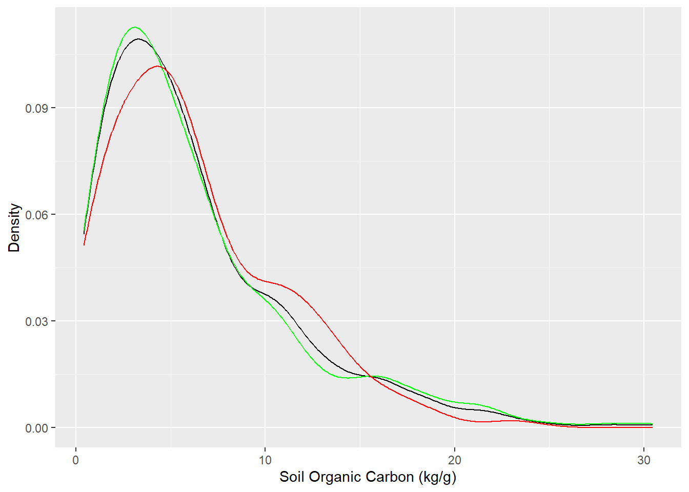
We will train a MLR model with selected predictors:
# Build the model
model <- lm(SOC ~., data = df_train)
summary(model)
Call:
lm(formula = SOC ~ ., data = df_train)

Residuals:
     Min       1Q   Median       3Q      Max
-10.6734  -2.1107  -0.3629   1.5035  16.1818

Coefficients:
                         Estimate Std. Error t value Pr(>|t|)
(Intercept)             6.8788435  2.9917952   2.299 0.022143 *
DEM                    -0.0012209  0.0007619  -1.602 0.110048
Slope                   0.1351551  0.0778406   1.736 0.083484 .
MAT                    -0.4057325  0.1032154  -3.931 0.000104 ***
MAP                     0.0073889  0.0018703   3.951 9.62e-05 ***
NDVI                    5.7768657  2.7201779   2.124 0.034471 *
NLCDHerbaceous         -1.8260715  0.9712617  -1.880 0.061014 .
NLCDPlanted/Cultivated -2.8156619  1.1251168  -2.503 0.012835 *
NLCDShrubland          -2.2404223  0.9175233  -2.442 0.015162 *
---
Signif. codes:  0 '***' 0.001 '**' 0.01 '*' 0.05 '.' 0.1 ' ' 1

Residual standard error: 3.878 on 316 degrees of freedom
Multiple R-squared:  0.4722,    Adjusted R-squared:  0.4589
F-statistic: 35.35 on 8 and 316 DF, p-value: < 2.2e-16We will use predict() function to predict SOC on test locations.
df_test$Pred.SOC <- model %>% predict(df_test)We will use Metrics package to compute several metrics to evaluate the model. All functions in the Metrics package take at least two arguments: actual and predicted.
Following metrices can be calculated using Metrics packages. It is recommended to use multiple evaluation metrics to assess the performance of the regression model as each metric provides a different perspective on the model’s accuracy.
RMSE<- Metrics::rmse(df_test$SOC, df_test$Pred.SOC)
MAE<- Metrics::mae(df_test$SOC, df_test$Pred.SOC)
MSE<- Metrics::mse(df_test$SOC, df_test$Pred.SOC)
MDAE<- Metrics::mdae(df_test$SOC, df_test$Pred.SOC)

# Print results
paste0("RMSE: ", round(RMSE,2))
[1] "RMSE: 3.74"paste0("MAE: ", round(MAE,2))[1] "MAE: 2.71"paste0("MSE: ", round(MSE,2))[1] "MSE: 13.99"paste0("MDAE: ", round(MDAE,2))[1] "MDAE: 1.96"We can plot observed and predicted values with fitted regression line with ggplot2
library(ggpmisc)
formula<-y~x

ggplot(df_test, aes(SOC,Pred.SOC)) +
  geom_point() +
  geom_smooth(method = "lm")+
  stat_poly_eq(use_label(c("eq", "adj.R2")), formula = formula) +
  ggtitle("Figure: Observed vs Predicted SOC ") +
  xlab("Observed") + ylab("Predicted") +
  scale_x_continuous(limits=c(0,20), breaks=seq(0, 20, 5))+
  scale_y_continuous(limits=c(0,20), breaks=seq(0, 20, 5)) +
  # Flip the bars
  theme(
    panel.background = element_rect(fill = "grey95",colour = "gray75",size = 0.5, linetype = "solid"),
    axis.line = element_line(colour = "grey"),
    plot.title = element_text(size = 14, hjust = 0.5),
    axis.title.x = element_text(size = 14),
    axis.title.y = element_text(size = 14),
    axis.text.x=element_text(size=13, colour="black"),
    axis.text.y=element_text(size=13,angle = 90,vjust = 0.5, hjust=0.5, colour='black'))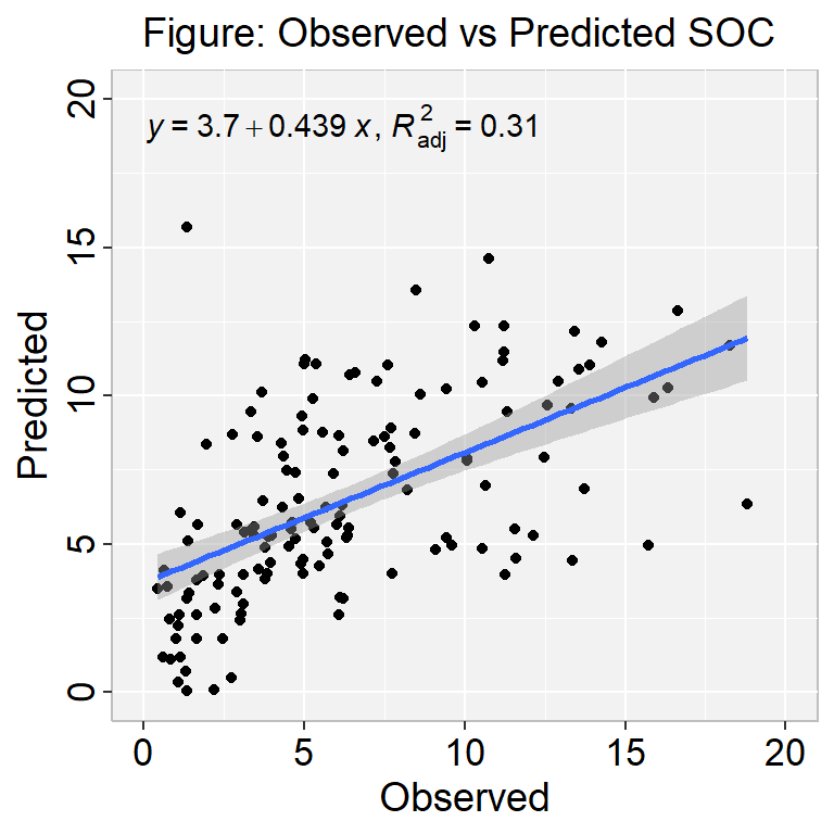
Cross-validation is a technique used to assess the performance and generalizability of a model. The basic idea is to split the data into several subsets, or folds, and use each subset in turn to evaluate the model trained on the remaining data.
Three major types of cross-validation techniques are usually use for model evaluation:
k-fold Cross Validation
Repeated k-fold Cross Validation
Leave One Out Cross Validation
The most common form of cross-validation is k-fold cross-validation, in which the data is divided into k non-overlapping folds of roughly equal size. The model is then trained on k-1 of the folds and evaluated on the remaining fold. This process is repeated k times, with each fold used as the validation set exactly once. The performance of the model is typically assessed by averaging the evaluation results across the k folds.
To perform cross-validation using the caret package, one can use the trainControl() function to specify the details of the cross-validation procedure, such as the number of folds and the type of resampling. Then, the train() function can be used to fit a model using the specified cross-validation procedure.
library(caret)
# Define training control
set.seed(123)
train.control <- trainControl(method = "cv", number = 10)
# Train the model
model.kfcv <- caret::train(SOC ~., data = df_train,
                           method = "lm",
                          trControl = train.control)
# Summarize the results
print(model.kfcv)
Linear Regression
325 samples
6 predictor
No pre-processing
Resampling: Cross-Validated (10 fold)
Summary of sample sizes: 292, 292, 292, 293, 293, 293, ...
Resampling results:
RMSE Rsquared MAE
3.878269 0.4431111 2.8183
Tuning parameter 'intercept' was held constant at a value of TRUEIt is similar to k-fold cross-validation, but the process is repeated multiple times with different random splits of the data. In k-fold cross-validation, the data is divided into k equally sized folds, and the model is trained and tested k times, with each fold being used once as the testing data and the remaining folds as training data. The average of these k performance measures is then used as an estimate of the model’s performance.
The following example uses 10-fold cross validation with 3 repeats:
set.seed(123)
train.control <- trainControl(method = "repeatedcv",
                              number = 10, repeats = 5)
# Train the model
model.rkfcv <- train(SOC ~., data = df_train, method = "lm",
               trControl = train.control)
# Summarize the results
print(model.rkfcv)
Linear Regression
325 samples
6 predictor
No pre-processing
Resampling: Cross-Validated (10 fold, repeated 5 times)
Summary of sample sizes: 292, 292, 292, 293, 293, 293, ...
Resampling results:
RMSE Rsquared MAE
3.902973 0.4660419 2.824213
Tuning parameter 'intercept' was held constant at a value of TRUELeave One Out Cross Validation (LOOCV) is a type of cross-validation method used in statistical analysis and machine learning to evaluate the performance of a model. In LOOCV, the data is split into training and testing sets in such a way that each observation is used as a testing sample exactly once.
The LOOCV process involves removing one observation from the data set and training the model on the remaining n-1 observations. The removed observation is then used as the test set, and the performance of the model is evaluated on this single observation. This process is repeated for each observation in the data set, resulting in n performance measures. The average of these performance measures is then used as an estimate of the model’s performance.
The advantage of the LOOCV method is that we make use all data points reducing potential bias. However, the process is repeated as many times as there are data points, resulting to a higher execution time when n is extremely large.
# Define training control
train.control <- trainControl(method = "LOOCV")
# Train the model
model.loocv <- train(SOC ~., data = df_train, method = "lm",
               trControl = train.control)
# Summarize the results
print(model.loocv)
Linear Regression
325 samples
6 predictor
No pre-processing
Resampling: Leave-One-Out Cross-Validation
Summary of sample sizes: 324, 324, 324, 324, 324, 324, ...
Resampling results:
RMSE Rsquared MAE
3.952533 0.4370173 2.828391
Tuning parameter 'intercept' was held constant at a value of TRUEBootstrap validation is a resampling technique used to estimate the uncertainty of a model’s performance.
# Define training control
train.control <- trainControl(method = "boot", number = 100)
# Train the model
model.boot <- train(SOC ~., data = df_train, method = "lm",
               trControl = train.control)
# Summarize the results
print(model.boot)
Linear Regression
325 samples
6 predictor
No pre-processing
Resampling: Bootstrapped (100 reps)
Summary of sample sizes: 325, 325, 325, 325, 325, 325, ...
Resampling results:
RMSE Rsquared MAE
4.0037 0.4227783 2.871766
Tuning parameter 'intercept' was held constant at a value of TRUECreate a R-Markdown documents (name homework_08.rmd) in this project and do all Tasks using the data shown below.
Submit all codes and output as a HTML document (homework_08.html) before class of next week.
tidyverse, rsample, caret, Metrics, ggpmisc
Download the data and save in your project directory. Use read_csv to load the data in your R-session. For example:
df<-read_csv(“bd_arsenic_data.csv”))
SAs: Soil Arenic
WAs: Groundwater As
WP: Groundwater P
WFe: Groundwater Fe
WEc: Groundwater Ec
WpH: Groundwater pH
SAoFe: Oxalate Extractable
SpH: Soil pH
SEc: Soil Ec
SOC: Soil Organic Carbon
SAND: Sand
SILT: Silt
CLAY: Clay
SP: Soil pH
ELEV: Elevation
Year_Irrig: Year of Irrigation
DIS_STW: Distance from STW
Land_types
Split the into training (70%) and test-data (30%) with stratified random sampling in landtypes
Create a density plot SAs for all, train, and test data.
Fit a MLR model with train data and make prediction on test data.
Calculate RMSE, MAE, MSE and MDAE with Metrics package
Plot predicted and Observed SOC, show the R2 and equation on plot.
Perform K-fold cross validation with caret package