Code
library(sf)
library(terra)
library(tidyverse)
library(rgdal)
Vector attribute manipulation involves working with the attribute data associated with geographic features in vector datasets. This process allows you to modify, aggregate, transform, and analyze the non-spatial information linked to each feature. In R, you can use packages like sf and dplyr from the tidyverse to perform attribute manipulation on vector data. When working with spatial data within the tidyverse framework, the sf package (Simple Features) plays a central role. This package seamlessly integrates spatial geometries with attribute manipulation using the familiar syntax of the dplyr and tidyr packages from the tidyverse. This integration makes it easy to work with both the spatial and attribute aspects of your vector data.
Here are some common tasks related to vector attribute manipulation you can accomplish:
Filtering: Selecting specific features based on certain criteria from the attribute data.
Attribute Calculation: Creating or modifying new attributes using mathematical operations or functions.
Grouping and Aggregation: Summarizing data by grouping features based on attribute values.
Sorting: Ordering features based on attribute values.
Joining: Combining attributes from different datasets based on a common identifier.
Attribute Transformation: Applying functions to attribute values to transform them.
String Manipulation: Modifying text attributes using string functions.
Conditional Updating: Updating attributes based on certain conditions.
Reshaping: Changing the attribute data structure (e.g., comprehensive to long format).
library(sf)
library(terra)
library(tidyverse)
library(rgdal)In this exercise we will use district-wise rice production data of Bangladesh.
Rice production by district of Bangladesh (bd_district_rice_production_2018_2019_BTM.shp)
Upazila shape file of Bangladesh (bd_upzila_BTM.shp)
CSV file of Upazila wise Poverty data (bd_poverty.csv)
The data can be found here for download.
We will use sf::st_read() to the data directly from GitHub:
# SFDF: Simple feature datafrme
SFDF = sf::st_read("/vsicurl/https://github.com//zia207/r-colab/raw/main/Data/Bangladesh//Shapefiles/bd_district_rice_production_2018_2019_BTM.shp")
Reading layer `bd_district_rice_production_2018_2019_BTM' from data source
`/vsicurl/https://github.com//zia207/r-colab/raw/main/Data/Bangladesh//Shapefiles/bd_district_rice_production_2018_2019_BTM.shp'
using driver `ESRI Shapefile'
Simple feature collection with 64 features and 19 fields
Geometry type: MULTIPOLYGON
Dimension: XY
Bounding box: xmin: 298487.8 ymin: 278578.1 xmax: 778101.8 ymax: 946939.2
Projected CRS: +proj=tmerc +lat_0=0 +lon_0=90 +k=0.9996 +x_0=500000 +y_0=-2000000 +datum=WGS84 +units=m +no_defsclass(SFDF)[1] "sf" "data.frame"You can use dplyr::glimps() to explore the attribute tables associated with shape file:
dplyr::glimpse(SFDF)Rows: 64
Columns: 20
$ Shape_Leng <dbl> 5.358126, 4.167970, 7.713625, 10.091155, 4.289236, 3.598531…
$ Shape_Area <dbl> 0.40135919, 0.11780114, 0.19522826, 0.17081236, 0.26009774,…
$ ADM2_EN <chr> "Bandarban", "Barguna", "Barisal", "Bhola", "Bogra", "Braha…
$ ADM2_PCODE <chr> "BD2003", "BD1004", "BD1006", "BD1009", "BD5010", "BD2012",…
$ ADM2_REF <chr> NA, NA, NA, NA, NA, NA, NA, NA, NA, NA, "Coxs Bazar", NA, N…
$ ADM2ALT1EN <chr> NA, NA, NA, NA, NA, NA, NA, NA, NA, NA, NA, NA, NA, NA, NA,…
$ ADM2ALT2EN <chr> NA, NA, NA, NA, NA, NA, NA, NA, NA, NA, NA, NA, NA, NA, NA,…
$ ADM1_EN <chr> "Chittagong", "Barisal", "Barisal", "Barisal", "Rajshahi", …
$ ADM1_PCODE <chr> "BD20", "BD10", "BD10", "BD10", "BD50", "BD20", "BD20", "BD…
$ ADM0_EN <chr> "Bangladesh", "Bangladesh", "Bangladesh", "Bangladesh", "Ba…
$ ADM0_PCODE <chr> "BD", "BD", "BD", "BD", "BD", "BD", "BD", "BD", "BD", "BD",…
$ date <chr> "2015/01/01", "2015/01/01", "2015/01/01", "2015/01/01", "20…
$ validOn <chr> "2020/11/13", "2020/11/13", "2020/11/13", "2020/11/13", "20…
$ ValidTo <chr> NA, NA, NA, NA, NA, NA, NA, NA, NA, NA, NA, NA, NA, NA, NA,…
$ DISTRICT_I <chr> "BD2003", "BD1004", "BD1006", "BD1009", "BD5010", "BD2012",…
$ YEAR <chr> "2018-2019", "2018-2019", "2018-2019", "2018-2019", "2018-2…
$ Aus <dbl> 23672, 11650, 38239, 172102, 57385, 20992, 26286, 97581, 10…
$ Aman <dbl> 26210, 116802, 208723, 423522, 467997, 133161, 79413, 43574…
$ Boro <dbl> 24253, 256997, 195101, 161003, 709612, 471298, 237576, 2449…
$ geometry <MULTIPOLYGON [m]> MULTIPOLYGON (((745209.5 47..., MULTIPOLYGON (…Division and district names are in this attribute table named “ADM1_EN” and “ADM2_EN, respectively. We will rename these attribute as”DIV_Name” and “DIST_Name” using dplyr::rename() function
SFDF.new<-dplyr::rename(SFDF, DIST_Name = ADM2_EN, DIV_Name = ADM1_EN) %>%
glimpse()
Rows: 64
Columns: 20
$ Shape_Leng <dbl> 5.358126, 4.167970, 7.713625, 10.091155, 4.289236, 3.598531…
$ Shape_Area <dbl> 0.40135919, 0.11780114, 0.19522826, 0.17081236, 0.26009774,…
$ DIST_Name <chr> "Bandarban", "Barguna", "Barisal", "Bhola", "Bogra", "Braha…
$ ADM2_PCODE <chr> "BD2003", "BD1004", "BD1006", "BD1009", "BD5010", "BD2012",…
$ ADM2_REF <chr> NA, NA, NA, NA, NA, NA, NA, NA, NA, NA, "Coxs Bazar", NA, N…
$ ADM2ALT1EN <chr> NA, NA, NA, NA, NA, NA, NA, NA, NA, NA, NA, NA, NA, NA, NA,…
$ ADM2ALT2EN <chr> NA, NA, NA, NA, NA, NA, NA, NA, NA, NA, NA, NA, NA, NA, NA,…
$ DIV_Name <chr> "Chittagong", "Barisal", "Barisal", "Barisal", "Rajshahi", …
$ ADM1_PCODE <chr> "BD20", "BD10", "BD10", "BD10", "BD50", "BD20", "BD20", "BD…
$ ADM0_EN <chr> "Bangladesh", "Bangladesh", "Bangladesh", "Bangladesh", "Ba…
$ ADM0_PCODE <chr> "BD", "BD", "BD", "BD", "BD", "BD", "BD", "BD", "BD", "BD",…
$ date <chr> "2015/01/01", "2015/01/01", "2015/01/01", "2015/01/01", "20…
$ validOn <chr> "2020/11/13", "2020/11/13", "2020/11/13", "2020/11/13", "20…
$ ValidTo <chr> NA, NA, NA, NA, NA, NA, NA, NA, NA, NA, NA, NA, NA, NA, NA,…
$ DISTRICT_I <chr> "BD2003", "BD1004", "BD1006", "BD1009", "BD5010", "BD2012",…
$ YEAR <chr> "2018-2019", "2018-2019", "2018-2019", "2018-2019", "2018-2…
$ Aus <dbl> 23672, 11650, 38239, 172102, 57385, 20992, 26286, 97581, 10…
$ Aman <dbl> 26210, 116802, 208723, 423522, 467997, 133161, 79413, 43574…
$ Boro <dbl> 24253, 256997, 195101, 161003, 709612, 471298, 237576, 2449…
$ geometry <MULTIPOLYGON [m]> MULTIPOLYGON (((745209.5 47..., MULTIPOLYGON (…You can apply the ggplot() function directly on the sf object to plot them.
SFDF.new %>%
  ggplot() +
  geom_sf(aes(fill = Aman)) +
  theme_minimal()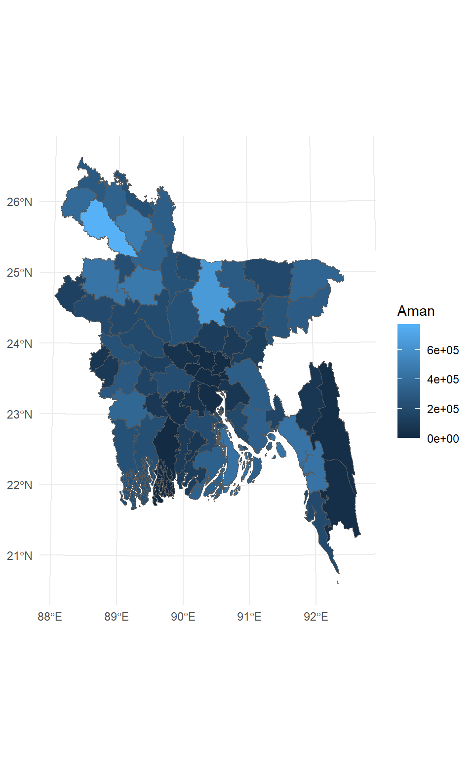
SFDF.new contains several non-geographic columns (and one geometry list column) with almost 64 rows representing the district of Bangladesh. The function sf::st_drop_geometry() keeps only the attributes data of an sf object, in other words removing its geometry. Dropping the geometry column before working with attribute data can be helpful to; data manipulation processes can run faster when they work only on the attribute data, and geometry columns are not always needed.
DF<-st_drop_geometry(SFDF.new) %>%
  glimpse()
Rows: 64
Columns: 19
$ Shape_Leng <dbl> 5.358126, 4.167970, 7.713625, 10.091155, 4.289236, 3.598531…
$ Shape_Area <dbl> 0.40135919, 0.11780114, 0.19522826, 0.17081236, 0.26009774,…
$ DIST_Name <chr> "Bandarban", "Barguna", "Barisal", "Bhola", "Bogra", "Braha…
$ ADM2_PCODE <chr> "BD2003", "BD1004", "BD1006", "BD1009", "BD5010", "BD2012",…
$ ADM2_REF <chr> NA, NA, NA, NA, NA, NA, NA, NA, NA, NA, "Coxs Bazar", NA, N…
$ ADM2ALT1EN <chr> NA, NA, NA, NA, NA, NA, NA, NA, NA, NA, NA, NA, NA, NA, NA,…
$ ADM2ALT2EN <chr> NA, NA, NA, NA, NA, NA, NA, NA, NA, NA, NA, NA, NA, NA, NA,…
$ DIV_Name <chr> "Chittagong", "Barisal", "Barisal", "Barisal", "Rajshahi", …
$ ADM1_PCODE <chr> "BD20", "BD10", "BD10", "BD10", "BD50", "BD20", "BD20", "BD…
$ ADM0_EN <chr> "Bangladesh", "Bangladesh", "Bangladesh", "Bangladesh", "Ba…
$ ADM0_PCODE <chr> "BD", "BD", "BD", "BD", "BD", "BD", "BD", "BD", "BD", "BD",…
$ date <chr> "2015/01/01", "2015/01/01", "2015/01/01", "2015/01/01", "20…
$ validOn <chr> "2020/11/13", "2020/11/13", "2020/11/13", "2020/11/13", "20…
$ ValidTo <chr> NA, NA, NA, NA, NA, NA, NA, NA, NA, NA, NA, NA, NA, NA, NA,…
$ DISTRICT_I <chr> "BD2003", "BD1004", "BD1006", "BD1009", "BD5010", "BD2012",…
$ YEAR <chr> "2018-2019", "2018-2019", "2018-2019", "2018-2019", "2018-2…
$ Aus <dbl> 23672, 11650, 38239, 172102, 57385, 20992, 26286, 97581, 10…
$ Aman <dbl> 26210, 116802, 208723, 423522, 467997, 133161, 79413, 43574…
$ Boro <dbl> 24253, 256997, 195101, 161003, 709612, 471298, 237576, 2449…Subsetting refers to selecting a subset of data from a larger dataset based on specific conditions or criteria. In other words, it involves extracting a portion of the data that meets specific requirements or characteristics. Subsetting is a common operation in data analysis that focuses on a specific subset of interest for further analysis, visualization, or processing.
In spatial data analysis, subsetting often involves selecting a subset of spatial features (points, lines, polygons) from a larger geographic dataset. This could include selecting specific geographic areas, isolating certain types of features, or narrowing down the dataset to a particular period or attribute value.
The [ operator can subset both rows and columns. Indices placed inside square brackets placed directly after a data frame object name specify the elements to keep. The key dplyr subsetting functions are filter() and slice() for subsetting rows and select() for subsetting columns. Both approaches preserve the spatial components of attribute data in sf objects.
SFDF.new[1:10] # Subset row by positionSimple feature collection with 64 features and 10 fields
Geometry type: MULTIPOLYGON
Dimension: XY
Bounding box: xmin: 298487.8 ymin: 278578.1 xmax: 778101.8 ymax: 946939.2
Projected CRS: +proj=tmerc +lat_0=0 +lon_0=90 +k=0.9996 +x_0=500000 +y_0=-2000000 +datum=WGS84 +units=m +no_defs
First 10 features:
Shape_Leng Shape_Area DIST_Name ADM2_PCODE ADM2_REF ADM2ALT1EN
1 5.358126 0.4013592 Bandarban BD2003 <NA> <NA>
2 4.167970 0.1178011 Barguna BD1004 <NA> <NA>
3 7.713625 0.1952283 Barisal BD1006 <NA> <NA>
4 10.091155 0.1708124 Bhola BD1009 <NA> <NA>
5 4.289236 0.2600977 Bogra BD5010 <NA> <NA>
6 3.598531 0.1705439 Brahamanbaria BD2012 <NA> <NA>
7 4.332182 0.1296815 Chandpur BD2013 <NA> <NA>
8 8.259337 0.3904653 Chittagong BD2015 <NA> <NA>
9 2.328542 0.1030781 Chuadanga BD4018 <NA> <NA>
10 3.833726 0.2728555 Comilla BD2019 <NA> <NA>
ADM2ALT2EN DIV_Name ADM1_PCODE ADM0_EN geometry
1 <NA> Chittagong BD20 Bangladesh MULTIPOLYGON (((745209.5 47...
2 <NA> Barisal BD10 Bangladesh MULTIPOLYGON (((487586.8 44...
3 <NA> Barisal BD10 Bangladesh MULTIPOLYGON (((556973.9 49...
4 <NA> Barisal BD10 Bangladesh MULTIPOLYGON (((579740 4170...
5 <NA> Rajshahi BD50 Bangladesh MULTIPOLYGON (((432389 7787...
6 <NA> Chittagong BD20 Bangladesh MULTIPOLYGON (((632854.6 68...
7 <NA> Chittagong BD20 Bangladesh MULTIPOLYGON (((562751.1 54...
8 <NA> Chittagong BD20 Bangladesh MULTIPOLYGON (((693227.3 45...
9 <NA> Khulna BD40 Bangladesh MULTIPOLYGON (((389280.6 63...
10 <NA> Chittagong BD20 Bangladesh MULTIPOLYGON (((605298.5 63...SFDF.new[, 15:20] # subset columns by positionSimple feature collection with 64 features and 5 fields
Geometry type: MULTIPOLYGON
Dimension: XY
Bounding box: xmin: 298487.8 ymin: 278578.1 xmax: 778101.8 ymax: 946939.2
Projected CRS: +proj=tmerc +lat_0=0 +lon_0=90 +k=0.9996 +x_0=500000 +y_0=-2000000 +datum=WGS84 +units=m +no_defs
First 10 features:
DISTRICT_I YEAR Aus Aman Boro geometry
1 BD2003 2018-2019 23672 26210 24253 MULTIPOLYGON (((745209.5 47...
2 BD1004 2018-2019 11650 116802 256997 MULTIPOLYGON (((487586.8 44...
3 BD1006 2018-2019 38239 208723 195101 MULTIPOLYGON (((556973.9 49...
4 BD1009 2018-2019 172102 423522 161003 MULTIPOLYGON (((579740 4170...
5 BD5010 2018-2019 57385 467997 709612 MULTIPOLYGON (((432389 7787...
6 BD2012 2018-2019 20992 133161 471298 MULTIPOLYGON (((632854.6 68...
7 BD2013 2018-2019 26286 79413 237576 MULTIPOLYGON (((562751.1 54...
8 BD2015 2018-2019 97581 435740 244972 MULTIPOLYGON (((693227.3 45...
9 BD4018 2018-2019 109585 89821 131195 MULTIPOLYGON (((389280.6 63...
10 BD2019 2018-2019 191367 316154 661982 MULTIPOLYGON (((605298.5 63...SFDF.new[1:10, 15:20] # subset rows and columns by positionSimple feature collection with 10 features and 5 fields
Geometry type: MULTIPOLYGON
Dimension: XY
Bounding box: xmin: 360715.6 ymin: 344101.5 xmax: 778101.8 ymax: 778758.6
Projected CRS: +proj=tmerc +lat_0=0 +lon_0=90 +k=0.9996 +x_0=500000 +y_0=-2000000 +datum=WGS84 +units=m +no_defs
DISTRICT_I YEAR Aus Aman Boro geometry
1 BD2003 2018-2019 23672 26210 24253 MULTIPOLYGON (((745209.5 47...
2 BD1004 2018-2019 11650 116802 256997 MULTIPOLYGON (((487586.8 44...
3 BD1006 2018-2019 38239 208723 195101 MULTIPOLYGON (((556973.9 49...
4 BD1009 2018-2019 172102 423522 161003 MULTIPOLYGON (((579740 4170...
5 BD5010 2018-2019 57385 467997 709612 MULTIPOLYGON (((432389 7787...
6 BD2012 2018-2019 20992 133161 471298 MULTIPOLYGON (((632854.6 68...
7 BD2013 2018-2019 26286 79413 237576 MULTIPOLYGON (((562751.1 54...
8 BD2015 2018-2019 97581 435740 244972 MULTIPOLYGON (((693227.3 45...
9 BD4018 2018-2019 109585 89821 131195 MULTIPOLYGON (((389280.6 63...
10 BD2019 2018-2019 191367 316154 661982 MULTIPOLYGON (((605298.5 63...We use to create a another SFDF object by subsetting columns by name, and “geometry” column will automatically retain in this new sf object
SFDF.subset<-SFDF.new[, c('DIST_Name', 'DIV_Name', 'YEAR', 'Aus', 'Aman', 'Boro')] %>%
  glimpse()
Rows: 64
Columns: 7
$ DIST_Name <chr> "Bandarban", "Barguna", "Barisal", "Bhola", "Bogra", "Braham…
$ DIV_Name <chr> "Chittagong", "Barisal", "Barisal", "Barisal", "Rajshahi", "…
$ YEAR <chr> "2018-2019", "2018-2019", "2018-2019", "2018-2019", "2018-20…
$ Aus <dbl> 23672, 11650, 38239, 172102, 57385, 20992, 26286, 97581, 109…
$ Aman <dbl> 26210, 116802, 208723, 423522, 467997, 133161, 79413, 435740…
$ Boro <dbl> 24253, 256997, 195101, 161003, 709612, 471298, 237576, 24497…
$ geometry <MULTIPOLYGON [m]> MULTIPOLYGON (((745209.5 47..., MULTIPOLYGON ((…You can apply dplyr::filter() function to extract all districts under the “Rangpur,” “Rajshahi” divisions.
SFDF.subset %>%
  filter(DIV_Name %in% c("Rangpur", "Rajshahi")) %>%
  glimpse()
Rows: 16
Columns: 7
$ DIST_Name <chr> "Bogra", "Dinajpur", "Gaibandha", "Joypurhat", "Kurigram", "…
$ DIV_Name <chr> "Rajshahi", "Rangpur", "Rangpur", "Rajshahi", "Rangpur", "Ra…
$ YEAR <chr> "2018-2019", "2018-2019", "2018-2019", "2018-2019", "2018-20…
$ Aus <dbl> 57385, 20324, 6157, 471, 3692, 14134, 179648, 18043, 138418,…
$ Aman <dbl> 467997, 770155, 349760, 218127, 314620, 239059, 443820, 1914…
$ Boro <dbl> 709612, 681567, 479310, 290082, 477747, 179177, 816283, 2754…
$ geometry <MULTIPOLYGON [m]> MULTIPOLYGON (((432389 7787..., MULTIPOLYGON ((…You may also use dplyr::select() to select columns by name or position.
SFDF.subset %>%
  select(DIST_Name, Aman) %>%
  plot()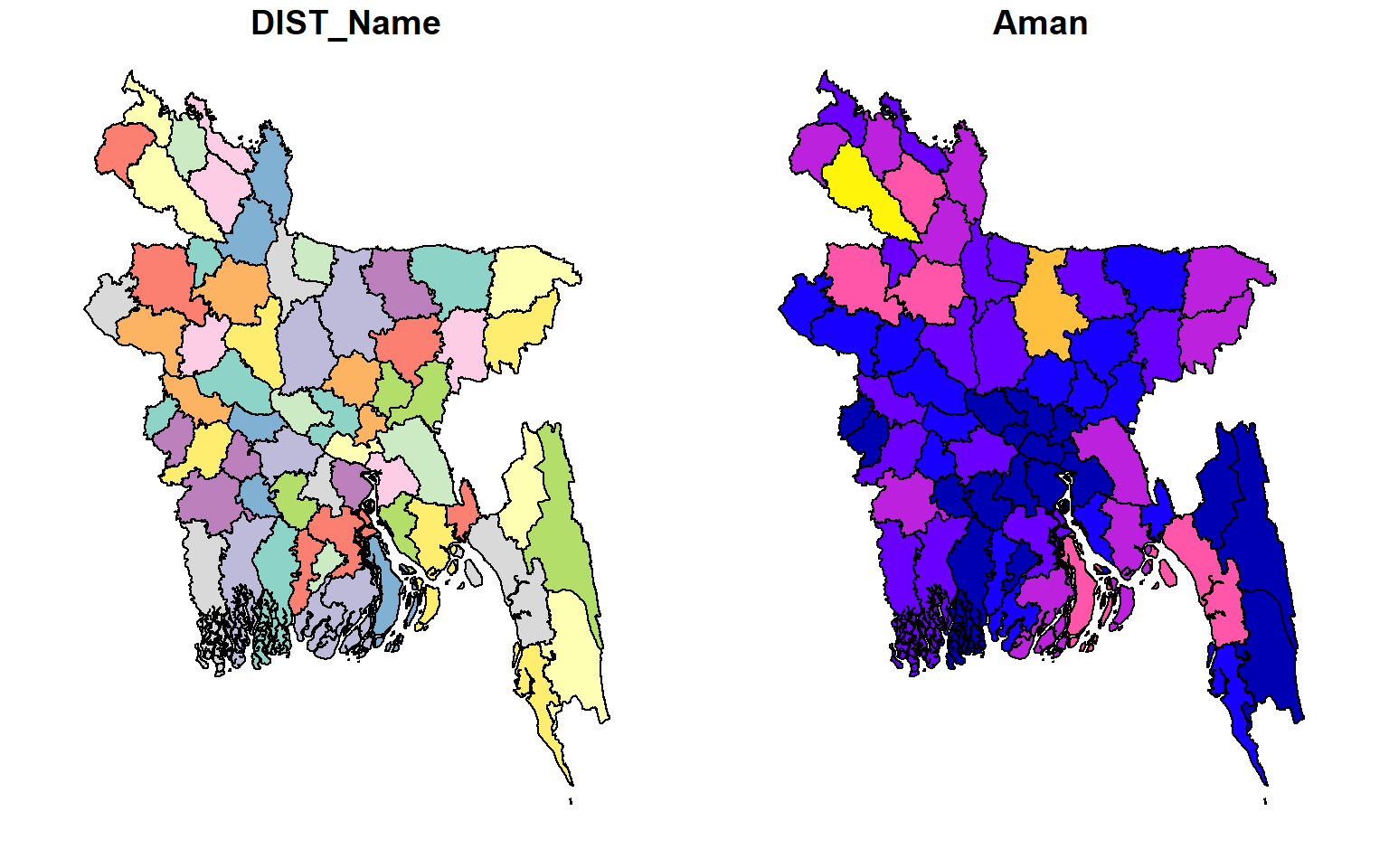
You can also apply dplyr::filter and dplyr::select together to create a new sf object and then plot it using the ggplot() function:
SFDF.subset %>%
  filter(DIV_Name %in% c("Rangpur", "Rajshahi")) %>%
  select(DIST_Name, Aman) %>%
  ggplot() +
  geom_sf(aes(fill = Aman)) +
  theme_minimal()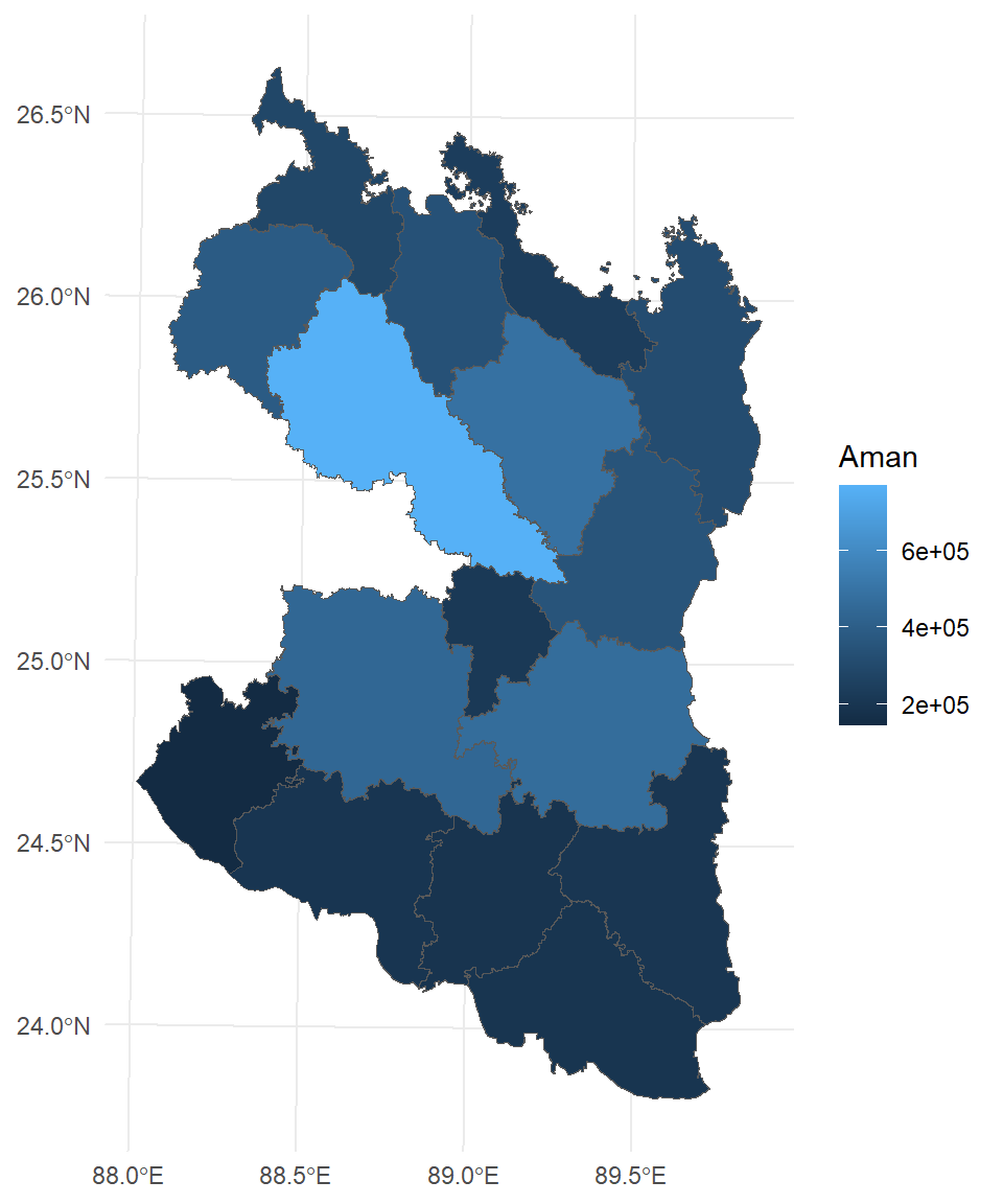
We can keep only rows matching the given criteria; for example, keep the districts where Boro production is lower than the mean.
 SFDF.new %>%
  filter(Boro < mean(SFDF.new$Boro)) %>%
    ggplot() +
    geom_sf(aes(fill = Boro)) +
    theme_minimal()+
ggtitle("District where Boro Production < Mean") 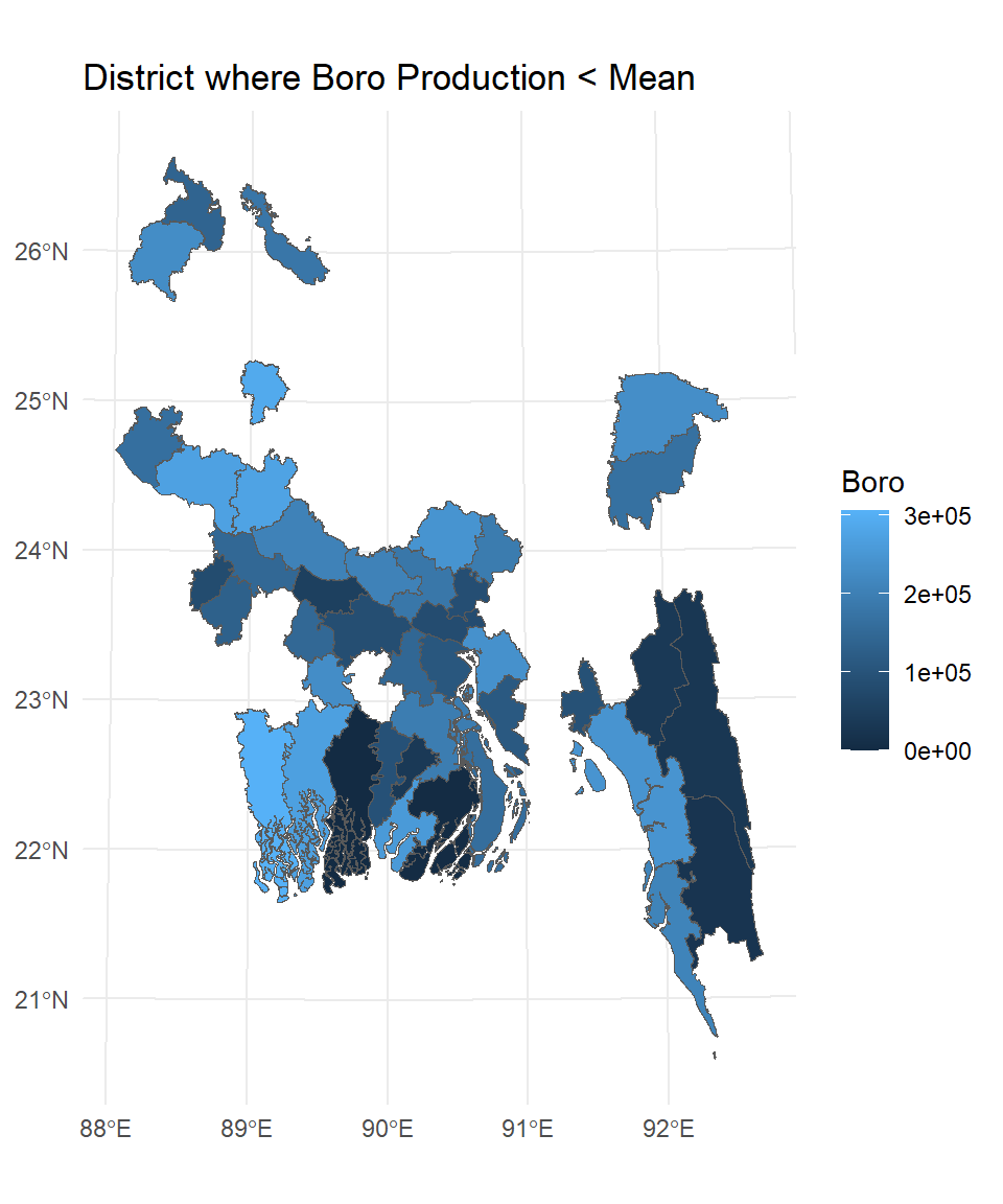
Vector attribute aggregation involves summarizing or calculating statistics from attribute data associated with geographic features in a vector dataset. This process allows you to condense and analyze the attribute information for specific groups, areas, or conditions within your spatial data.
An example of attribute aggregation is calculating total Boro production per division based on the district-level data
SFDF.new %>%
  group_by(DIV_Name) %>%
  summarise(MT=sum(Boro)) %>%
  ggplot() +
  geom_sf(aes(fill = MT)) +
  theme_minimal() +
  ggtitle("Total Boro Production (MT) by Divisions")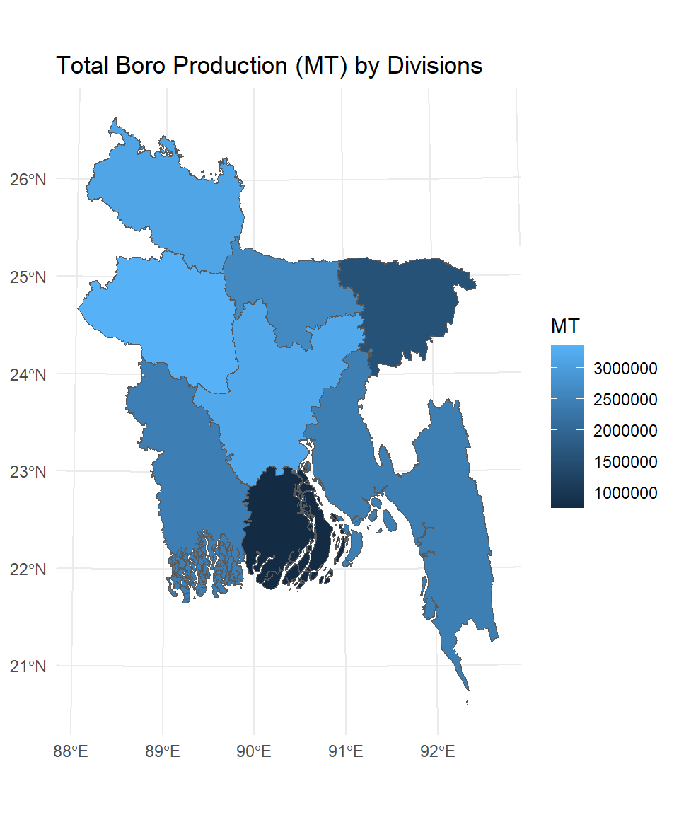
What is going on in terms of the geometries? Behind the scenes, summarize() combine the geometries and dissolve the boundaries.
Vector attribute joining combines attribute data from two or more datasets based on a common identifier or key. This process allows you to enhance or enrich your data by adding information from one dataset to another. In spatial data analysis, attribute joining is often used to combine non-spatial data with spatial features based on a shared attribute, such as an ID or name. In R, you can use packages like sf and dplyr from the tidyverse to perform attribute joins on vector data. In this exercise, we will combine poverty percentage data with Bangladesh’s upazila shape file.
# define file from my github
urlfile.poverty = "https://github.com//zia207/r-colab/raw/main/Data/Bangladesh/bd_poverty.csv"
poverty<-read_csv(url(urlfile.poverty)) %>%
  glimpse()
Rows: 544
Columns: 2
$ ADM3_PCODE <chr> "BD400108", "BD400114", "BD400134", "BD201358", "BD400…
$ POVERTY_PERCENT <dbl> 35.9, 50.0, 36.4, 42.5, 46.1, 41.9, 46.5, 41.1, 48.0, …# SFDF: Simple feature datafrme
SFDF.upz = sf::st_read("/vsicurl/https://github.com//zia207/r-colab/raw/main/Data/Bangladesh//Shapefiles/bd_upzila_BTM.shp")Reading layer `bd_upzila_BTM' from data source
`/vsicurl/https://github.com//zia207/r-colab/raw/main/Data/Bangladesh//Shapefiles/bd_upzila_BTM.shp'
using driver `ESRI Shapefile'
Simple feature collection with 544 features and 16 fields
Geometry type: MULTIPOLYGON
Dimension: XY
Bounding box: xmin: 298487.8 ymin: 278578.1 xmax: 778101.8 ymax: 946939.2
Projected CRS: +proj=tmerc +lat_0=0 +lon_0=90 +k=0.9996 +x_0=500000 +y_0=-2000000 +datum=WGS84 +units=m +no_defsFollowing R code will first 1) select some column, 2) rename them 3) join the poverty data with a common ID (ADM3_PCODE) with dplyr::inner_join() function , 4) finally plot the poverty percentage using ggplot()
SFDF.upz %>%
  select(ADM1_EN, ADM2_EN, ADM3_EN, ADM3_PCODE) %>%
  rename(DIST_Name = ADM2_EN, DIV_Name = ADM1_EN, UPZ_Name =ADM3_EN ) %>%
  inner_join(poverty) %>%
  ggplot() +
  geom_sf(aes(fill =  POVERTY_PERCENT )) +
  theme_minimal() +
  ggtitle("Poverty (%)")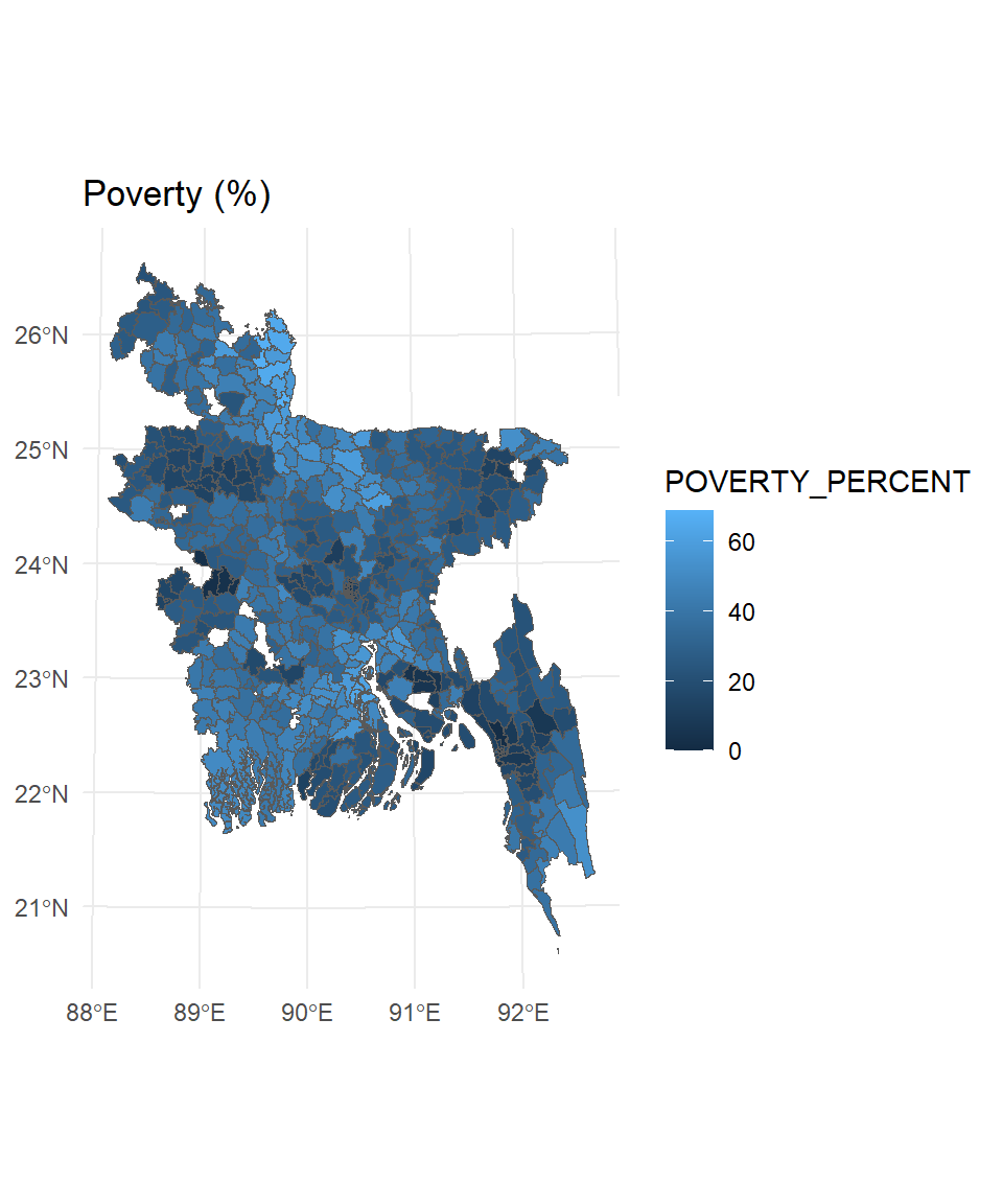
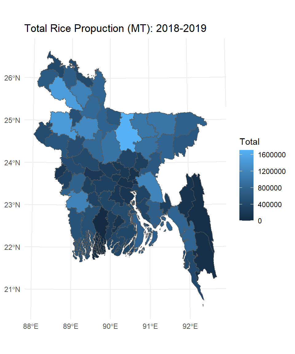
Creating attributes in spatial data involves adding new columns or variables to the attribute table associated with geographic features in a vector dataset. These attributes can store additional information, calculated values, or metadata that provide context and meaning to the spatial features.
For example, we will calculate total rice production for each district and create a new attribute name “Total_Production”. For this we need to add Aus, Aman and Boro attributes.
Using base R, we can type:
SFDF.new$Total <-SFDF.new$Aus+SFDF.new$Aman+SFDF.new$Boro
glimpse(SFDF.new)
Rows: 64
Columns: 21
$ Shape_Leng <dbl> 5.358126, 4.167970, 7.713625, 10.091155, 4.289236, 3.598531…
$ Shape_Area <dbl> 0.40135919, 0.11780114, 0.19522826, 0.17081236, 0.26009774,…
$ DIST_Name <chr> "Bandarban", "Barguna", "Barisal", "Bhola", "Bogra", "Braha…
$ ADM2_PCODE <chr> "BD2003", "BD1004", "BD1006", "BD1009", "BD5010", "BD2012",…
$ ADM2_REF <chr> NA, NA, NA, NA, NA, NA, NA, NA, NA, NA, "Coxs Bazar", NA, N…
$ ADM2ALT1EN <chr> NA, NA, NA, NA, NA, NA, NA, NA, NA, NA, NA, NA, NA, NA, NA,…
$ ADM2ALT2EN <chr> NA, NA, NA, NA, NA, NA, NA, NA, NA, NA, NA, NA, NA, NA, NA,…
$ DIV_Name <chr> "Chittagong", "Barisal", "Barisal", "Barisal", "Rajshahi", …
$ ADM1_PCODE <chr> "BD20", "BD10", "BD10", "BD10", "BD50", "BD20", "BD20", "BD…
$ ADM0_EN <chr> "Bangladesh", "Bangladesh", "Bangladesh", "Bangladesh", "Ba…
$ ADM0_PCODE <chr> "BD", "BD", "BD", "BD", "BD", "BD", "BD", "BD", "BD", "BD",…
$ date <chr> "2015/01/01", "2015/01/01", "2015/01/01", "2015/01/01", "20…
$ validOn <chr> "2020/11/13", "2020/11/13", "2020/11/13", "2020/11/13", "20…
$ ValidTo <chr> NA, NA, NA, NA, NA, NA, NA, NA, NA, NA, NA, NA, NA, NA, NA,…
$ DISTRICT_I <chr> "BD2003", "BD1004", "BD1006", "BD1009", "BD5010", "BD2012",…
$ YEAR <chr> "2018-2019", "2018-2019", "2018-2019", "2018-2019", "2018-2…
$ Aus <dbl> 23672, 11650, 38239, 172102, 57385, 20992, 26286, 97581, 10…
$ Aman <dbl> 26210, 116802, 208723, 423522, 467997, 133161, 79413, 43574…
$ Boro <dbl> 24253, 256997, 195101, 161003, 709612, 471298, 237576, 2449…
$ geometry <MULTIPOLYGON [m]> MULTIPOLYGON (((745209.5 47..., MULTIPOLYGON (…
$ Total <dbl> 74135, 385449, 442063, 756627, 1234994, 625451, 343275, 778…Alternatively, we can use one of dplyr functions mutate() which adds new columns at the penultimate position in the sf object (the last one is reserved for the geometry):
SFDF.new  %>%
  mutate(Total = Aus+Aman+Boro) %>%
  glimpse()
Rows: 64
Columns: 21
$ Shape_Leng <dbl> 5.358126, 4.167970, 7.713625, 10.091155, 4.289236, 3.598531…
$ Shape_Area <dbl> 0.40135919, 0.11780114, 0.19522826, 0.17081236, 0.26009774,…
$ DIST_Name <chr> "Bandarban", "Barguna", "Barisal", "Bhola", "Bogra", "Braha…
$ ADM2_PCODE <chr> "BD2003", "BD1004", "BD1006", "BD1009", "BD5010", "BD2012",…
$ ADM2_REF <chr> NA, NA, NA, NA, NA, NA, NA, NA, NA, NA, "Coxs Bazar", NA, N…
$ ADM2ALT1EN <chr> NA, NA, NA, NA, NA, NA, NA, NA, NA, NA, NA, NA, NA, NA, NA,…
$ ADM2ALT2EN <chr> NA, NA, NA, NA, NA, NA, NA, NA, NA, NA, NA, NA, NA, NA, NA,…
$ DIV_Name <chr> "Chittagong", "Barisal", "Barisal", "Barisal", "Rajshahi", …
$ ADM1_PCODE <chr> "BD20", "BD10", "BD10", "BD10", "BD50", "BD20", "BD20", "BD…
$ ADM0_EN <chr> "Bangladesh", "Bangladesh", "Bangladesh", "Bangladesh", "Ba…
$ ADM0_PCODE <chr> "BD", "BD", "BD", "BD", "BD", "BD", "BD", "BD", "BD", "BD",…
$ date <chr> "2015/01/01", "2015/01/01", "2015/01/01", "2015/01/01", "20…
$ validOn <chr> "2020/11/13", "2020/11/13", "2020/11/13", "2020/11/13", "20…
$ ValidTo <chr> NA, NA, NA, NA, NA, NA, NA, NA, NA, NA, NA, NA, NA, NA, NA,…
$ DISTRICT_I <chr> "BD2003", "BD1004", "BD1006", "BD1009", "BD5010", "BD2012",…
$ YEAR <chr> "2018-2019", "2018-2019", "2018-2019", "2018-2019", "2018-2…
$ Aus <dbl> 23672, 11650, 38239, 172102, 57385, 20992, 26286, 97581, 10…
$ Aman <dbl> 26210, 116802, 208723, 423522, 467997, 133161, 79413, 43574…
$ Boro <dbl> 24253, 256997, 195101, 161003, 709612, 471298, 237576, 2449…
$ geometry <MULTIPOLYGON [m]> MULTIPOLYGON (((745209.5 47..., MULTIPOLYGON (…
$ Total <dbl> 74135, 385449, 442063, 756627, 1234994, 625451, 343275, 778…SFDF.new %>%
mutate(Total = Aus+Aman+Boro) %>%
ggplot() +
geom_sf(aes(fill = Total )) +
theme_minimal() +
ggtitle("Total Rice Propuction (MT): 2018-2019")