Code
library (terra)
library(sf)
library (rgdal)
library(tidyverse)
library(classInt)
library(RColorBrewer)
library(raster)
library(gridExtra)
library(rasterVis)
library(whitebox)
library(tmap)
Geomorphometric analysis refers to the study of the quantitative characteristics and measurements of the Earth’s surface and its landforms using digital elevation models (DEMs) and other geospatial data. This type of analysis aims to extract valuable information about terrain features, slope, aspect, curvature, and other geomorphic attributes. Geomorphometric analysis is widely used in various fields, including geography, geology, environmental science, hydrology, and landscape ecology. It helps researchers and professionals better understand landforms, erosion processes, hydrological patterns, and landscape evolution.
library (terra)
library(sf)
library (rgdal)
library(tidyverse)
library(classInt)
library(RColorBrewer)
library(raster)
library(gridExtra)
library(rasterVis)
library(whitebox)
library(tmap)We will use 30 M SRTM elevation one small area in Bandarban district, Bangladesh and the data can be found here for download.
## Input data
dem <- "G:/My Drive/Data/Bangladesh/Raster/aoi_dtm_dem_BTM.tif"
dem
[1] "G:/My Drive/Data/Bangladesh/Raster/aoi_dtm_dem_BTM.tif"rgb.palette <- colorRampPalette(c('lightblue',"blue","green","yellow","red", "red3"),
space = "rgb")
dem_ras <- terra::rast(dem)
spplot(dem_ras, main="30m SRTM DEM", col.regions=rgb.palette(100))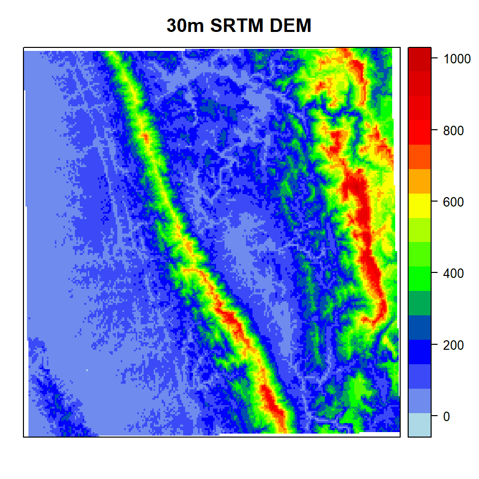
tmap_mode("view")
dem_ras <- terra::rast(dem)
tm_shape(dem_ras)+
  tm_raster(style = "cont", palette = "PuOr", legend.show = TRUE)+
tm_scale_bar()This tool calculates slope gradient (i.e. slope steepness in degrees, radians, or percent) for each grid cell in an input digital elevation model (DEM). The user must specify the name of the input DEM (--dem) and the output raster image. The Z conversion factor is only important when the vertical and horizontal units are not the same in the DEM. When this is the case, the algorithm will multiply each elevation in the DEM by the Z conversion factor.
# define output
slope.degree <- "G:/My Drive/Data/Bangladesh/Raster/Geomorph/slope_deg.tif"
# calculate  slope degree
wbt_slope(dem, slope.degree, units = 'degrees')
# convert to terra raster
slope.degree_ras <- terra::rast(slope.degree)
# plot
p1=spplot(slope.degree_ras,
        main= "Slope (Degree)",
col.regions=rgb.palette(100))# define output
slope.percent <- "G:/My Drive/Data/Bangladesh/Raster/Geomorph/slope_percent.tif"
# calculate percent slope
wbt_slope(dem, slope.percent, units = 'percent')
# convert to terra raster
slope.percent_ras <- terra::rast(slope.percent)
# plot
p2=spplot(slope.percent_ras,
main= "Slope (Percent)",
col.regions=rgb.palette(100))# define output
slope.radians <- "G:/My Drive/Data/Bangladesh/Raster/Geomorph/slope_radians.tif"
# calculate slope - radians
wbt_slope(dem, slope.radians, units = 'radians')
# convert to terra raster
slope.radians_ras <- terra::rast(slope.radians)
# plot
p3=spplot(slope.radians_ras,
main= "Slope (Radians)",
col.regions=rgb.palette(100))gridExtra::grid.arrange(p1,p2,p3, ncol=3)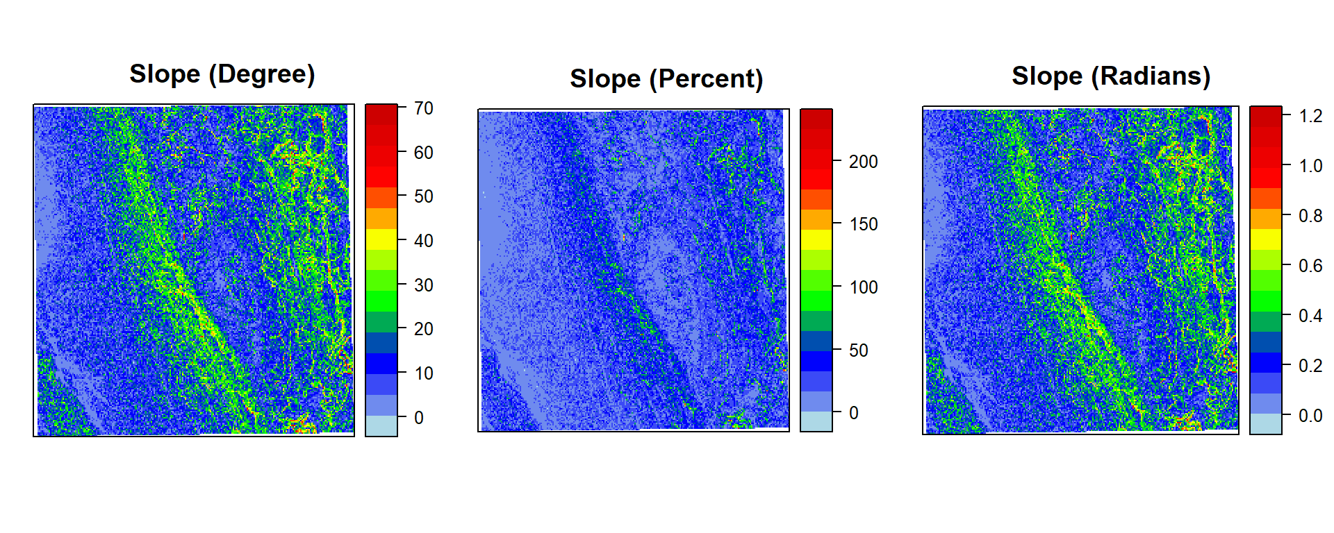
This tool calculates slope aspect (i.e. slope orientation in degrees clockwise from north) for each grid cell in an input digital elevation model (DEM).
# define output
aspect <- "G:/My Drive/Data/Bangladesh/Raster/Geomorph/aspect.tif"
# calculate aspect
wbt_aspect(dem, aspect)
# convert to terra raster
aspect_ras <- terra::rast(aspect)# plot
spplot(aspect_ras,
main= "Aspect",
col.regions=rgb.palette(100))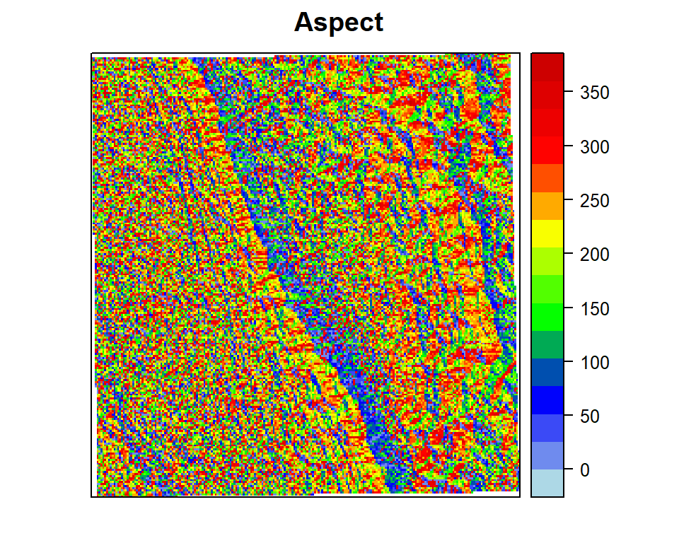
Th wbt_hillshade tool performs a hillshade operation (also called shaded relief) on an input digital elevation model (DEM). The user must specify the name of the input DEM and the output hillshade image name.
# define output
hillshade <- "G:/My Drive/Data/Bangladesh/Raster/Geomorph/hillshade.tif"
# calculate hillshade
wbt_hillshade(dem, hillshade, azimuth=315.0, altitude=30.0, )
# convert to terra raster
hillshade_ras <- terra::rast(hillshade)# plot
tm_shape(hillshade_ras)+
tm_raster(style = "cont", palette = "-Greys", legend.show = FALSE)+
tm_scale_bar()stars object downsampled to 1025 by 975 cells. See tm_shape manual (argument raster.downsample)The terrain ruggedness index (TRI) is a measure of local topographic relief. The TRI calculates the root-mean-square-deviation (RMSD) for each grid cell in a digital elevation model (DEM), calculating the residuals (i.e. elevation differences) between a grid cell and its eight neighbours.
# define output
ruggedness<- "G:/My Drive/Data/Bangladesh/Raster/Geomorph/ruggedness.tif"
# calculate ruggedness
wbt_ruggedness_index(dem, ruggedness)
# convert to terra raster
ruggedness_ras <- terra::rast(ruggedness)# plot
spplot(ruggedness_ras,
main= "Ruggedness Index",
col.regions=rgb.palette(100))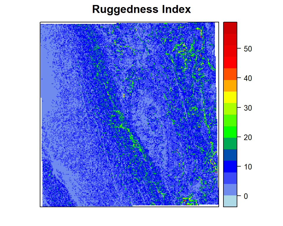
Curvature, in the context of geomorphometry and geography, refers to a fundamental geomorphic attribute that describes the rate of change of slope or the bending of the Earth’s surface at a specific point. It provides information about the shape and morphology of landforms, helping researchers understand the local surface characteristics and terrain features.
This tool calculates the profile (or vertical) curvature, or the rate of change in slope along a flow line, from a digital elevation model (DEM). It is the curvature of a normal section having a common tangent line with a slope line at a given point on the surface (Florinsky, 2017). This variable has an unbounded range that can take either positive or negative values. Positive values of the index are indicative of flow acceleration while negative profile curvature values indicate flow deceleration. Profile curvature is measured in units of m-1.
# define output
profile_curvature<- "G:/My Drive/Data/Bangladesh/Raster/Geomorph/profile_curvature.tif"
# calculate profile curvature
wbt_profile_curvature(dem, profile_curvature, log= TRUE)
# convert to terra raster
profile_curvature_ras <- terra::rast(profile_curvature)# plot
spplot(profile_curvature_ras,
main= "Profile Curvature",
col.regions=rgb.palette(100))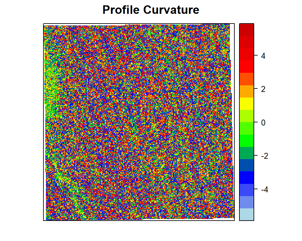
This tool calculates the plan (or contour) curvature from a digital elevation model (DEM). Plan curvature is the curvature of a contour line at a given point on the topographic surface (Florinsky, 2017). This variable has an unbounded range that can take either positive or negative values. Positive values of the index are indicative of flow divergence while negative plan curvature values indicate flow convergence. Thus plan curvature is similar to tangential curvature, although the literature suggests that the latter is more numerically stable (Wilson, 2018). Plan curvature is measured in units of m-1.
# define output
plan_curvature<- "G:/My Drive/Data/Bangladesh/Raster/Geomorph/plan_curvature.tif"
# calculate plan curvature
wbt_plan_curvature(dem, plan_curvature, log= TRUE)
# convert to terra raster
plan_curvature_ras <- terra::rast(plan_curvature)# plot
spplot(plan_curvature_ras,
main= "Plan Curvature",
col.regions=rgb.palette(100))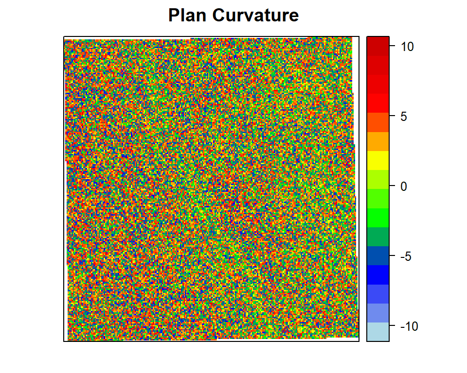
This tool calculates the total curvature from a digital elevation model (DEM). Total curvature measures the curvature of the topographic surface rather than the curvature of a line across the surface in some direction (Wilson, 2018). Total curvature can be positive or negative, with zero curvature indicating that the surface is either flat or the convexity in one direction is balanced by the concavity in another direction, as would occur at a saddle point. Total curvature is measured in units of m-1.
# define output
total_curvature<- "G:/My Drive/Data/Bangladesh/Raster/Geomorph/total_curvature.tif"
# calculate total_curvature
wbt_total_curvature(dem, total_curvature, log= TRUE)
# convert to terra raster
total_curvature_ras <- terra::rast(total_curvature)# plot
spplot(total_curvature_ras,
main= "Total Curvature",
col.regions=rgb.palette(100))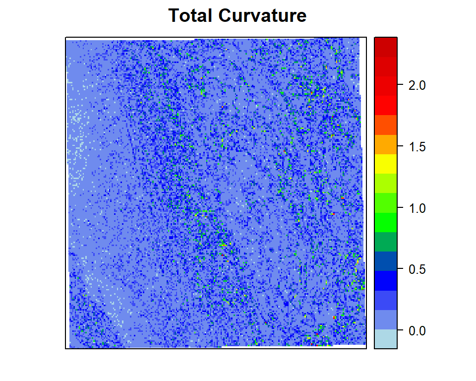
This tool calculates the tangential (or horizontal) curvature, which is the curvature of an inclined plane perpendicular to both the direction of flow and the surface (Gallant and Wilson, 2000). Alternatively, it could be described as the curvature of a normal section tangential to a contour line at a given point of the topographic surface (Florinsky, 2017). This variable has an unbounded range that can be either positive or negative. Positive values are indicative of flow divergence while negative tangential curvature values indicate flow convergence. Thus tangential curvature is similar to plan curvature, although the literature suggests that the former is more numerically stable (Wilson, 2018). Tangential curvature is measured in units of m-1.
# define output
tangential_curvature<- "G:/My Drive/Data/Bangladesh/Raster/Geomorph/tangential_curvature.tif"
# calculate plan curvature
wbt_tangential_curvature(dem, tangential_curvature, log= TRUE)
# convert to terra raster
tangential_curvature_ras <- terra::rast(tangential_curvature)# plot
spplot(tangential_curvature_ras,
main= "Tangential curvature",
col.regions=rgb.palette(100))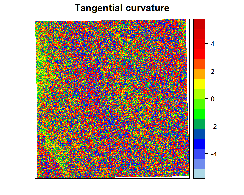
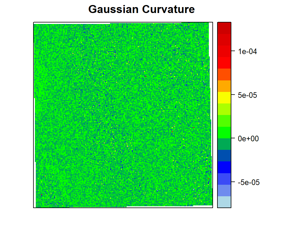
This tool calculates the Gaussian curvature from a digital elevation model (DEM). Gaussian curvature is the product of maximal and minimal curvatures, and retains values in each point of the topographic surface after its bending without breaking, stretching, and compressing (Florinsky, 2017). Gaussian curvature is measured in units of m-2.
# define output
gaussian_curvature<- "G:/My Drive/Data/Bangladesh/Raster/Geomorph/gaussian_curvature.tif"
# calculate plan curvature
wbt_gaussian_curvature(dem, gaussian_curvature)
# convert to terra raster
gaussian_curvature_ras <- terra::rast(gaussian_curvature)# plot
spplot(gaussian_curvature_ras,
main= "Gaussian Curvature",
col.regions=rgb.palette(100))