1. Generalized Linear Regression (Gaussian)

In this tutorial, we will explore Generalized Linear Models (GLMs), focusing on the Gaussian distribution, one of the most commonly used in GLMs. These models extend linear regression, enabling us to analyze a wider range of data types and relationships. We will start with an overview of GLM structure, discussing the random component (distribution), systematic component (predictors), and link function (mean transformation). We will establish a solid understanding of the fundamentals by constructing a GLM model using synthetic data without built-in R packages. Next, we will fit a GLM using R’s glm() function, interpreting the output to assess the influence of predictors and their statistical significance. We will also evaluate model performance and use R’s visualization libraries to create helpful graphics to interpret our results. This tutorial will equip you with the theoretical foundation and practical skills to confidently apply Gaussian GLMs in R for various statistical modeling applications.

Overview

Generalized Linear Models (GLMs) with a Gaussian distribution are useful for modeling relationships between a continuous response variable and one or more explanatory variables when the error terms are normally distributed. This is a generalization of linear regression where the assumptions of Gaussian distribution apply. Here’s an outline of the mathematical background and the steps to fit such a model.

  1. Model Specification:

    • The model assumes that the dependent variable \(Y\) follows a Gaussian (normal) distribution:

      \[ Y \sim \mathcal{N}(\mu, \sigma^2) \]

    • Here, \(\mu\) (the mean of \(Y\)) is modeled as a linear combination of predictors \(X\), so:

      \[ \mu = X\beta \]

    • Therefore, the model can be written as:

      \[ Y = X\beta + \epsilon \]

      where \(\epsilon \sim \mathcal{N}(0, \sigma^2)\) represents the error term.

  2. Link Function:

    • The identity link function is used for Gaussian models, meaning that we assume \(E[Y | X] = X\beta\).
  3. Parameter Estimation:

    • The coefficients \(\beta\) are estimated by minimizing the sum of squared errors (SSE):

    \[ \text{SSE} = \sum_{i=1}^n (Y_i - X_i\beta)^2 \]

    • The solution is given by:

    \[\beta = (X^T X)^{-1} X^T Y\]

    • This is derived using calculus (specifically, by taking the derivative of SSE with respect to ( \(\beta\) ), setting it to zero, and solving).
  4. Prediction:

    • Once ( \(\beta\) ) is estimated, we can predict new values of \(Y\) as:

    \[ \hat{Y} = X\beta \]

  5. Interpretation:

    • Each coefficient \(\beta_j\) represents the change in \(Y\) for a one-unit increase in \(X_j\), holding other predictors constant.

GLM Regression Model from Scratch

To fit a Generalized Linear Model (GLM) with a Gaussian distribution in R without using any packages, we’ll walk through each step, from generating synthetic data to estimating the model parameters and creating a summary statistics table. Let’s break down each mathematical concept and translate it into R code.

Steps to Fit the Model in R are below:

Generate Synthetic Data

We’ll start by generating synthetic data with four covariates and a continuous response variable.

  1. Define Number of Observations: ( \(n\) = 100 ).

  2. Generate Covariates (\(X_1, X_2, X_3, X_4\) ) from a normal distribution with mean ( 0 ) and standard deviation ( 1 ).

  3. Specify True Coefficients: Choose known values for the coefficients (\(\beta_0\) = 5 ) (intercept), (\(\beta\) = [1.5, -2.0, 0.5, 3.0]).

  4. Generate the Response Variable ($Y) using the formula:

    \[ Y = \beta\_0 + \beta\_1 X_1 + \beta\_2 X_2 + \beta\_3 X_3 + \beta\_4 X_4 + \epsilon\]

where \(\epsilon \sim N(0, 1)\) represents Gaussian noise.

Code
# Step 1: Generate Synthetic Data
set.seed(42)
n <- 100

# Generate covariates
X1 <- rnorm(n, 0, 1)
X2 <- rnorm(n, 0, 1)
X3 <- rnorm(n, 0, 1)
X4 <- rnorm(n, 0, 1)

# Define true coefficients
beta_0 <- 5
beta_true <- c(1.5, -2.0, 0.5, 3.0)

# Generate response variable Y
Y <- beta_0 + beta_true[1]*X1 + beta_true[2]*X2 + beta_true[3]*X3 + beta_true[4]*X4 + rnorm(n, 0, 1)

Define the Design Matrix ( \(X\) )

To estimate the coefficients, we need a design matrix (\(X\)) that includes an intercept term. The matrix (\(X\)) will look like this:

\[ X = \begin{bmatrix} 1 & X_{1,1} & X_{1,2} & X_{1,3} & X_{1,4} \\ 1 & X_{2,1} & X_{2,2} & X_{2,3} & X_{2,4} \\ \vdots & \vdots & \vdots & \vdots & \vdots \\ 1 & X_{n,1} & X_{n,2} & X_{n,3} & X_{n,4} \end{bmatrix} \]

where the first column is all ones for the intercept, and the remaining columns are values of the covariates ( $X_1, X_2, X_3, X_4 $) for each observation.

Code
# Step 2: Define Design Matrix X with Intercept
X <- cbind(1, X1, X2, X3, X4)
head(X)
               X1         X2         X3           X4
[1,] 1  1.3709584  1.2009654 -2.0009292 -0.004620768
[2,] 1 -0.5646982  1.0447511  0.3337772  0.760242168
[3,] 1  0.3631284 -1.0032086  1.1713251  0.038990913
[4,] 1  0.6328626  1.8484819  2.0595392  0.735072142
[5,] 1  0.4042683 -0.6667734 -1.3768616 -0.146472627
[6,] 1 -0.1061245  0.1055138 -1.1508556 -0.057887335

Estimate Coefficients Using the Normal Equation

For Gaussian GLMs, estimating the coefficients ( \(\beta\)) reduces to solving the Normal Equation:

\[\hat{\beta} = (X^T X)^{-1} X^T Y\]

Compute \(X^TX\): This is the matrix product of the transpose of (\(X\)) with (\(X\)).

Compute \((X^T X)^{-1}\): Invert the result from step 1.

Compute \(X^T Y\): This is the product of the transpose of \(X\) and the response vector (\(Y\) ).

Solve for \(\hat{\beta}\): Multiply the results from step 2 with step 3 to obtain the estimated coefficients.

Code
# Step 3: Estimate Coefficients Using Normal Equation
XtX <- t(X) %*% X
XtX_inv <- solve(XtX)
XtY <- t(X) %*% Y
beta_hat <- XtX_inv %*% XtY
beta_hat
         [,1]
    4.8602898
X1  1.5859543
X2 -2.1482949
X3  0.5901182
X4  3.2139250

Calculate Fitted Values and Residuals

  • **Fitted Values \(\hat{Y}\): Using the estimated coefficients \(\hat{\beta}\), calculate the fitted values as:

\[ \hat{Y} = X \hat{\beta}\]

  • Residuals: Calculate the residuals, which represent the difference between the observed values \(Y\) and fitted values \(\hat{Y}\):

\[ \text{residuals} = Y - \hat{Y} \]

Code
# Step 4: Calculate Fitted Values and Residuals
Y_hat <- X %*% beta_hat
residuals <- Y - Y_hat
head(residuals)
            [,1]
[1,]  1.71618876
[2,] -0.71880623
[3,] -0.09868479
[4,]  0.06564803
[5,] -0.41685869
[6,] -0.71816280

Compute Mean Squared Error (MSE) and Variance of Residuals

The Mean Squared Error (MSE) measures the average of the squared residuals:

\[\text{MSE} = \frac{1}{n}\sum_{i=1}^{n} (Y_i - \hat{Y}_i)^2\]

The variance of the residuals, used for calculating standard errors, is given by:

\[ \text{Var(residuals)} = \frac{1}{n - p - 1}\sum_{i=1}^{n} (Y_i - \hat{Y}_i)^2\]

where (\(p\) ) is the number of covariates (in our case, ( p = 4)

Code
# Step 5: Calculate MSE and Variance of Residuals
mse <- mean(residuals^2)
variance_residuals <- sum(residuals^2) / (n - length(beta_hat))

cat("Mean Squared Error (MSE):", mse, "\n")
Mean Squared Error (MSE): 0.965506 
Code
cat("Variance Residuals:", variance_residuals, "\n")
Variance Residuals: 1.016322 

Calculate Standard Errors and t-values for Coefficients

  • Standard Errors: The standard error for each coefficient ( _j ) is given by:

\[ \text{Std Error}(\hat{\beta}*j) =* \sqrt{\text{Var(residuals)} \times [ (X^T X)^{-1} ]_{jj} } \]

where ( \([(X^T X)^{-1}]{jj}\) is the \(j-th\) diagonal element of the inverse of \(X^T X\)$

  • t-values: The t-value for each coefficient tests the null hypothesis that the coefficient is zero. It is calculated as:

\[t\text{-value} = \frac{\hat{\beta}_j}{\text{Std Error}(\hat{\beta}_j)}\]

Code
# Step 6: Calculate Standard Errors and t-values
std_errors <- sqrt(variance_residuals * diag(XtX_inv))
t_values <- beta_hat / std_errors

Create a Summary Table

Code
# Step 7: Create Summary Table
summary_table <- data.frame(
  Coefficient = beta_hat,
  `Std Error` = std_errors,
  `t-value` = t_values
)

# Display Results
print(summary_table)
   Coefficient  Std.Error    t.value
     4.8602898 0.10141388  47.925291
X1   1.5859543 0.09864811  16.076884
X2  -2.1482949 0.11244878 -19.104652
X3   0.5901182 0.10104992   5.839868
X4   3.2139250 0.11603554  27.697764

Model Performance

Evaluating a Generalized Linear Model (GLM) involves several key metrics to assess its fit and predictive power. Below, I’ll outline the main evaluation metrics commonly used for a Gaussian GLM, along with their calculations.

Evaluation Matrix

  1. Mean Squared Error (MSE):

    • Measures the average of the squares of the errors (residuals), which is the difference between the predicted and actual values.

    \[ \text{MSE} = \frac{1}{n} \sum_{i=1}^{n} (Y_i - \hat{Y}_i)^2 \]

  2. Root Mean Squared Error (RMSE):

    • The square root of MSE, providing an error metric in the same units as the response variable.

    \[ \text{RMSE} = \sqrt{\text{MSE}} \]

  3. Mean Absolute Error (MAE):

    • Measures the average absolute errors, providing a straightforward interpretation of the average error magnitude.

    \[ \text{MAE} = \frac{1}{n} \sum_{i=1}^{n} |Y_i - \hat{Y}_i|\]

  4. R-squared (\(R^2\)):

    • Indicates the proportion of variance in the response variable that can be explained by the model.

    \[ R^2 = 1 - \frac{\text{SS}_{\text{res}}}{\text{SS}_{\text{tot}}} \]

    where:

\[ \text{SS}_{\text{res}} = \sum_{i=1}^{n} (Y_i - \hat{Y}_i)^2 \] \[ \text{SS}_{\text{tot}} = \sum_{i=1}^{n} (Y_i - \bar{Y})^2 \]

  1. Adjusted R-squared:

    • Adjusts the R-squared value based on the number of predictors in the model, providing a more accurate assessment when comparing models.

    \[ \text{Adjusted } R^2 = 1 - \left( \frac{(1 - R^2)(n - 1)}{n - p - 1} \right) \]

    where \(p\) is the number of predictors.

  2. Akaike Information Criterion (AIC):

    • Provides a measure of model quality that accounts for the number of parameters.

    \[ \text{AIC} = n \log\left(\frac{\text{SS}_{\text{res}}}{n}\right) + 2p \]

  3. Bayesian Information Criterion (BIC):

    • Similar to AIC but with a larger penalty for models with more parameters.

    \[ \text{BIC} = n \log\left(\frac{\text{SS}_{\text{res}}}{n}\right) + p \log(n)\]

Code
### Calculating the Metrics

# Observed Values Y: The actual response values.
# Fitted Values Y_hat: The predicted response values from the model.
# umber of Observations, n: 100
# Number of Predictors, p : 4 (excluding the intercept)."

n <- 100  # Number of observations
p <- 4    # Number of predictors (X1, X2, X3, X4)

# Step 1: Calculate MSE
MSE <- mean((Y - Y_hat)^2)

# Step 2: Calculate RMSE
RMSE <- sqrt(MSE)

# Step 3: Calculate MAE
MAE <- mean(abs(Y - Y_hat))

# Step 4: Calculate R-squared
SS_res <- sum((Y - Y_hat)^2)  # Residual sum of squares
SS_tot <- sum((Y - mean(Y))^2)  # Total sum of squares
R_squared <- 1 - (SS_res / SS_tot)

# Step 5: Calculate Adjusted R-squared
adjusted_R_squared <- 1 - ((1 - R_squared) * (n - 1)) / (n - p - 1)

# Step 6: Calculate AIC
AIC <- n * log(SS_res / n) + 2 * (p + 1)  # +1 for the intercept

# Step 7: Calculate BIC
BIC <- n * log(SS_res / n) + (p + 1) * log(n)  # +1 for the intercept

# Print results
cat("Mean Squared Error (MSE):", MSE, "\n")
Mean Squared Error (MSE): 0.965506 
Code
cat("Root Mean Squared Error (RMSE):", RMSE, "\n")
Root Mean Squared Error (RMSE): 0.9826017 
Code
cat("Mean Absolute Error (MAE):", MAE, "\n")
Mean Absolute Error (MAE): 0.7571292 
Code
cat("R-squared:", R_squared, "\n")
R-squared: 0.9372941 
Code
cat("Adjusted R-squared:", adjusted_R_squared, "\n")
Adjusted R-squared: 0.9346539 
Code
cat("Akaike Information Criterion (AIC):", AIC, "\n")
Akaike Information Criterion (AIC): 6.489706 
Code
cat("Bayesian Information Criterion (BIC):", BIC, "\n")
Bayesian Information Criterion (BIC): 19.51556 

K-fold Cross-validation

  • Split the Data: Randomly divide the dataset into \(K\) equal-sized folds.

  • Training and Testing:

    • For each fold, use \(k-1\) folds for training the model and the remaining fold for testing.

    • Repeat this process \(k\) times, ensuring that each fold serves as the test set once.

  • Model Fitting: Fit the GLM on the training set for each iteration.

  • Prediction: Use the fitted model to make predictions on the test set.

  • Performance Metrics: Calculate evaluation metrics (e.g., MSE, RMSE, MAE, etc.) for each fold.

  • Aggregate Results: Compute the average and standard deviation of the performance metrics across all folds

Code
# K-Fold Cross-Validation

k <- 10  # Number of folds
folds <- cut(seq(1, n), breaks = k, labels = FALSE)
cv_mse <- numeric(k)  # Store MSE for each fold

for (i in 1:k) {
  # Split data into training and validation sets
  test_indices <- which(folds == i, arr.ind = TRUE)
  train_indices <- setdiff(1:n, test_indices)
  
  # Training set
  X_train <- X[train_indices, ]
  Y_train <- Y[train_indices]
  
  # Testing set
  X_test <- X[test_indices, ]
  Y_test <- Y[test_indices]
  
  # Fit the model on training data
  XtX_train <- t(X_train) %*% X_train
  XtX_inv_train <- solve(XtX_train)
  XtY_train <- t(X_train) %*% Y_train
  beta_hat_train <- XtX_inv_train %*% XtY_train
  
  # Predict on test set
  Y_pred <- X_test %*% beta_hat_train
  
  # Calculate MSE for this fold
  cv_mse[i] <- mean((Y_test - Y_pred)^2)
}

# Average MSE across folds
average_cv_mse <- mean(cv_mse)
cat("Average K-Fold Cross-Validation MSE:", average_cv_mse, "\n")
Average K-Fold Cross-Validation MSE: 1.120817 

1:1 plot Predicted vs Observed Values

Code
# Plot Observed vs Predicted Values
plot(Y, Y_hat, main = "Observed vs Predicted Values", 
     xlab = "Observed Y", 
     ylab = "Predicted Y", pch = 16, col = "grey")
abline(0, 1, col = "black", lwd = 2)  # Add a 1:1 line for reference

GLM Regression Model in R

To fit a Generalized Linear Model (GLM) with a Gaussian distribution using the glm() function from base R, we’ll go through each step, including data exploration, fitting the model, interpretation and evaluate the model performance with a holdout test data set.

Install Required R Packages

We will install and load the necessary R packages for data manipulation, visualization, and model fitting. The packages include tidyverse, boot, margins, ggeffects, performance, sjPlot, patchwork, gt, gtsummary, jtools, report, Metrics, and metrica.

Code
# Packages List
packages <- c(
  "tidyverse",   # Includes readr, dplyr, ggplot2, etc.
  "plyr",
  "rstatix",
  "boot",
  "margins",
  "marginaleffects",
  "ggeffects",
  "performance",
  "ggpmisc",
  "sjPlot",
  "patchwork",
  "gt",
  "gtsummary",
  "jtools",
  "report",
  "Metrics",
  "metrica"
)
#| warning: false
#| error: false

# Install missing packages
new_packages <- packages[!(packages %in% installed.packages()[,"Package"])]
if(length(new_packages)) install.packages(new_packages)

# Verify installation
cat("Installed packages:\n")
print(sapply(packages, requireNamespace, quietly = TRUE))

Load R Packages

Code
# Load packages with suppressed messages
invisible(lapply(packages, function(pkg) {
  suppressPackageStartupMessages(library(pkg, character.only = TRUE))
}))
Code
# Check loaded packages
cat("Successfully loaded packages:\n")
Successfully loaded packages:
Code
print(search()[grepl("package:", search())])
 [1] "package:metrica"         "package:Metrics"        
 [3] "package:report"          "package:jtools"         
 [5] "package:gtsummary"       "package:gt"             
 [7] "package:patchwork"       "package:sjPlot"         
 [9] "package:ggpmisc"         "package:ggpp"           
[11] "package:performance"     "package:ggeffects"      
[13] "package:marginaleffects" "package:margins"        
[15] "package:boot"            "package:rstatix"        
[17] "package:plyr"            "package:lubridate"      
[19] "package:forcats"         "package:stringr"        
[21] "package:dplyr"           "package:purrr"          
[23] "package:readr"           "package:tidyr"          
[25] "package:tibble"          "package:ggplot2"        
[27] "package:tidyverse"       "package:stats"          
[29] "package:graphics"        "package:grDevices"      
[31] "package:utils"           "package:datasets"       
[33] "package:methods"         "package:base"           

Data

Our goal is to develop a GLM regression model to predict paddy soil arsenic (SAs) concentration using various irrigation water and soil properties. We have available data of 263 paired groundwater and paddy soil samples from arsenic contaminated areas in Tala Upazilla, Satkhira district, Bangladesh. This data was utilized in a publication titled “Factors Affecting Paddy Soil Arsenic Concentration in Bangladesh: Prediction and Uncertainty of Geostatistical Risk Mapping” which can be accessed via the this URL

Full data set is available for download can download from my Dropbox or from my Github accounts.

We will use read_csv() function of {readr} package to import data as a tidy data.

Code
# Load data
mf<-readr::read_csv("https://github.com/zia207/r-colab/raw/main/Data/Regression_analysis/bd_soil_arsenic.csv")
meta.as<-readr::read_csv("https://github.com/zia207/r-colab/raw/main/Data/Regression_analysis/bd_soil_arsenic_meta_data.csv") 
gt::gt(meta.as)
Variables Description
WAs Irrigation water Arsenic
WP Irrigation water P
WFe Irrigation water Fe
WEc Irrigation water Ec
WpH Irrigation water pH
WMg Irrigation water Mg
WNa Irrigation water Na
WCa Irrigation water Ca
WK Irrigation water K
WS Irrigation water S
SAs Soil Total As
SPAs Phosphate exchangeable As
SAOAs Oxalate extractable As
SAOFe Amorphous FeO
SpH Soil pH
SEc Soil Ec
SOC Soil Organic Carbon
Sand Sand Percent
Silt Silt Percent
Clay Caly Percent
SP Soil P
Elevation Elevation
Year_Irrigation Year of Irrigation
Dicstance_STW Distance from STW
Land_type Flooding landtype
Land_type_ID Flooding landtype ID

Summary Statistics

Code
mf |> 
  # select variables
  dplyr::select (WAs, WP, WFe,  
                WEc, WpH, SAoFe, SpH, SOC, 
                Sand, Silt, SP, Elevation, 
                Year_Irrigation, Distance_STW,
                SAs) |> 
  rstatix::get_summary_stats (type = "common")  
# A tibble: 15 × 10
   variable      n     min     max  median     iqr    mean      sd     se     ci
   <fct>     <dbl>   <dbl>   <dbl>   <dbl>   <dbl>   <dbl>   <dbl>  <dbl>  <dbl>
 1 WAs         263 1.1 e-2 4.58e-1 1.19e-1   0.1      0.13   0.079  0.005  0.01 
 2 WP          263 2.16e-1 2.70e+0 1.09e+0   0.456    1.11   0.368  0.023  0.045
 3 WFe         263 1.78e+0 1.10e+1 5.06e+0   2.64     5.29   1.97   0.121  0.239
 4 WEc         263 3.9 e-1 4.16e+0 1.08e+0   0.84     1.30   0.712  0.044  0.086
 5 WpH         263 6.58e+0 7.56e+0 7.01e+0   0.18     7.01   0.14   0.009  0.017
 6 SAoFe       263 1   e+3 4.94e+3 2.57e+3 565     2597.   626.    38.6   76.0  
 7 SpH         263 6.54e+0 8.71e+0 8.17e+0   0.35     8.12   0.309  0.019  0.038
 8 SOC         263 5.4 e-1 2.64e+0 1.35e+0   0.33     1.36   0.307  0.019  0.037
 9 Sand        263 4.9 e+0 2.79e+1 1.2 e+1   2.1     12.1    3.00   0.185  0.365
10 Silt        263 1.63e+1 7.01e+1 4.56e+1   6.75    44.5    8.03   0.495  0.975
11 SP          263 2.43e+0 5.23e+1 1.54e+1   3.61    15.6    5.9    0.364  0.716
12 Elevation   263 1   e+0 9   e+0 4   e+0   2        4.28   1.71   0.105  0.208
13 Year_Irr…   263 1   e+0 2   e+1 6   e+0   6        7.02   4.16   0.257  0.506
14 Distance…   263 3   e+0 4.5 e+1 9   e+0   5        9.50   6.14   0.378  0.745
15 SAs         263 4.7 e+0 5.18e+1 1.72e+1   9.35    17.9    7.39   0.456  0.897

Correlation Matrix

Code
mf |> 
  # select variables
  dplyr::select (WAs, WP, WFe,  
                WEc, WpH, SAoFe, SpH, SOC, 
                Sand, Silt, SP, Elevation, 
                Year_Irrigation, Distance_STW,
                SAs) |> 
  rstatix::cor_test (SAs)  
# A tibble: 14 × 8
   var1  var2               cor statistic        p conf.low conf.high method 
   <chr> <chr>            <dbl>     <dbl>    <dbl>    <dbl>     <dbl> <chr>  
 1 SAs   WAs              0.24      3.91  1.18e- 4  0.118      0.346  Pearson
 2 SAs   WP               0.15      2.48  1.38e- 2  0.0313     0.268  Pearson
 3 SAs   WFe              0.32      5.47  1.03e- 7  0.208      0.425  Pearson
 4 SAs   WEc              0.15      2.38  1.81e- 2  0.0251     0.262  Pearson
 5 SAs   WpH             -0.014    -0.232 8.17e- 1 -0.135      0.107  Pearson
 6 SAs   SAoFe           -0.11     -1.77  7.87e- 2 -0.227      0.0125 Pearson
 7 SAs   SpH              0.019     0.311 7.56e- 1 -0.102      0.140  Pearson
 8 SAs   SOC              0.34      5.81  1.79e- 8  0.227      0.441  Pearson
 9 SAs   Sand            -0.074    -1.21  2.29e- 1 -0.194      0.0470 Pearson
10 SAs   Silt            -0.26     -4.42  1.47e- 5 -0.373     -0.147  Pearson
11 SAs   SP               0.13      2.08  3.9 e- 2  0.00654    0.245  Pearson
12 SAs   Elevation       -0.34     -5.85  1.45e- 8 -0.443     -0.229  Pearson
13 SAs   Year_Irrigation  0.53     10.0   2.94e-20  0.434      0.610  Pearson
14 SAs   Distance_STW    -0.2      -3.32  1.04e- 3 -0.314     -0.0821 Pearson

Boxplot and Jitter Plots

Code
# Create a custom color 
rgb.palette <- colorRampPalette(c("red","yellow","green", "blue"),
space = "rgb")

# Create plot
ggplot(mf, aes(y=SAs, x=Land_type)) +
  geom_point(aes(colour=WAs),size = I(1.7),
             position=position_jitter(width=0.05, height=0.05)) +
  geom_boxplot(fill=NA, outlier.colour=NA) +
  labs(title="")+
  # Change figure orientation 
  coord_flip()+
  # add custom color plate and legend title
  scale_colour_gradientn(name="Water As (mg/kg)", colours =rgb.palette(10))+
  theme(legend.text = element_text(size = 10),legend.title = element_text(size = 12))+
  # add y-axis title and x-axis title leave blank
  labs(y="Soil As (mg/kg)", x = "")+ 
  # add plot title
  ggtitle("Soil As in relation to Water As in two Landtypes")+
  # customize plot themes
  theme(
        axis.line = element_line(colour = "black"),
        # plot title position at center
        plot.title = element_text(hjust = 0.5),
        # axis title font size
        axis.title.x = element_text(size = 12), 
        # X and  axis font size
        axis.text.y=element_text(size=10,vjust = 0.5, hjust=0.5, colour='black'),
        axis.text.x = element_text(size=12))

Data Processing

We will apply following operation before fit a GLM regression model.

  1. Feature engineering: Feature engineering is a vital task in the data preparation process for data analysis, particularly for machine learning models. It is the practice of creating new features from existing ones or transforming them to enhance the machine learning algorithm’s performance. Doing so makes achieving higher accuracy, better generalization, and a more straightforward interpretation of the model possible. Some standard techniques used in feature engineering include dimensionality reduction, feature scaling, and feature extraction. When performing feature engineering, it is essential to consider the data type, distribution, and target variable, among other factors.

We will create a new feature (Sand_Silt) by adding soil Silt and Sand percentage

  1. Convert to factors: As Land_type is categorical variable representing distinct categories rather than numerical values, we need to convert them into factors. This process will allow us to analyze and interpret the data more accurately, facilitating a better understanding of the underlying patterns and trends.

  2. Data normalization: It is a technique used in data analysis and machine learning. It involves adjusting numerical values to a standard range, usually between 0 and 1 or with a mean of 0 and a standard deviation of 1. This helps to improve the efficiency and accuracy of machine learning algorithms. Data normalization is important because it helps machine learning models work better. By standardizing the data, the models can more easily identify patterns and relationships in the data, which leads to better predictions and results.

Code
df <- mf |> 
  # select variables
  dplyr::select (WAs, WP, WFe,  
                WEc, WpH, SAoFe, SpH, SOC, 
                Sand, Silt, SP, Elevation, 
                Year_Irrigation, Distance_STW,
                Land_type, SAs) |> 
   # convert to factor
   dplyr::mutate_at(vars(Land_type), funs(factor))  |> 
   # create a variable
   dplyr::mutate (Silt_Sand = Silt+Sand)  |> 
   # drop two variables
   dplyr::select(-c(Silt,Sand)) |> 
   # relocate or organized variable
   dplyr::relocate(SAs, .after=Silt_Sand) |> 
   dplyr::relocate(Land_type, .after=Silt_Sand) |> 
   # normalize the all numerical features 
   dplyr::mutate_at(1:13,  funs((.-min(.))/max(.-min(.)))) |> 
   glimpse()
Rows: 263
Columns: 15
$ WAs             <dbl> 0.10738255, 0.10738255, 0.15212528, 0.24832215, 0.1364…
$ WP              <dbl> 0.21949255, 0.39387837, 0.44341522, 0.53523963, 0.3020…
$ WFe             <dbl> 0.1804348, 0.3423913, 0.8608696, 0.7391304, 0.3260870,…
$ WEc             <dbl> 0.16976127, 0.18037135, 0.26790451, 0.11671088, 0.2732…
$ WpH             <dbl> 0.4591837, 0.4897959, 0.2653061, 0.2755102, 0.3775510,…
$ SAoFe           <dbl> 0.3807107, 0.4238579, 0.2944162, 0.3807107, 0.2690355,…
$ SpH             <dbl> 0.5529954, 0.6129032, 0.6866359, 0.7050691, 0.5852535,…
$ SOC             <dbl> 0.5333333, 0.3428571, 0.3904762, 0.5095238, 0.3428571,…
$ SP              <dbl> 0.2277923, 0.2582715, 0.2628835, 0.2777221, 0.2360136,…
$ Elevation       <dbl> 0.250, 0.500, 0.375, 0.250, 0.500, 0.125, 0.125, 0.250…
$ Year_Irrigation <dbl> 0.68421053, 1.00000000, 0.47368421, 0.36842105, 0.4736…
$ Distance_STW    <dbl> 0.04761905, 0.07142857, 0.04761905, 0.11904762, 0.0476…
$ Silt_Sand       <dbl> 0.6139456, 0.5918367, 0.5731293, 0.5323129, 0.6462585,…
$ Land_type       <fct> MHL, MHL, MHL, MHL, MHL, MHL, MHL, MHL, MHL, MHL, MHL,…
$ SAs             <dbl> 29.10, 45.10, 23.20, 23.80, 26.00, 25.60, 26.30, 31.60…

Split Data

We will use the ddply() function of the {plyr} package to split soil carbon datainto homogeneous subgroups using stratified random sampling. This method involves dividing the population into strata and taking random samples from each stratum to ensure that each subgroup is proportionally represented in the sample. The goal is to obtain a representative sample of the population by adequately representing each stratum.

Code
seeds = 11076
tr_prop = 0.70
# training data (70% data)
train= ddply(df,.(Land_type),
                 function(., seed) { set.seed(seed); .[sample(1:nrow(.), trunc(nrow(.) * tr_prop)), ] }, seed = 101)
test = ddply(df, .(Land_type),
            function(., seed) { set.seed(seed); .[-sample(1:nrow(.), trunc(nrow(.) * tr_prop)), ] }, seed = 101)
Note

Stratified random sampling Stratified random sampling is a technique for selecting a representative sample from a population, where the sample is chosen in a way that ensures that certain subgroups within the population are adequately represented in the sample.

Fit a GLM Model

In the context of a GLM with continuous response variables, the focus is on regression problems where the dependent variable, which is being predicted, is continuous. This implies that the variable can take any value within a specific range, and the objective is to identify a correlation between the dependent variable and the independent variables that can be used to make accurate predictions.

To fta a GLM model with continuous response variables in R, we will use the glm() function with family=gaussian(link = "identity"). The SAs variable will be used as a response variable, while all the other variables in the train will serve as predictors.

Code
fit.glm<-glm(SAs~.,train, 
             family= gaussian(link = "identity")
             )  

Model Summary

The summary() function provides a summary of the fitted GLM model, including coefficients, standard errors, t-values, and p-values, among other statistics. This summary can help you interpret the relationship between the predictors and the response variable.

Code
summary(fit.glm)

Call:
glm(formula = SAs ~ ., family = gaussian(link = "identity"), 
    data = train)

Coefficients:
                Estimate Std. Error t value Pr(>|t|)    
(Intercept)       13.043      4.290   3.040 0.002742 ** 
WAs                5.260      2.799   1.879 0.061993 .  
WP                -3.333      2.919  -1.142 0.255110    
WFe                6.062      2.221   2.729 0.007029 ** 
WEc                1.989      2.239   0.888 0.375710    
WpH                1.982      3.182   0.623 0.534165    
SAoFe             -4.280      2.334  -1.834 0.068416 .  
SpH                1.082      3.171   0.341 0.733280    
SOC                2.615      3.228   0.810 0.419111    
SP                 7.594      3.099   2.451 0.015286 *  
Elevation         -2.457      2.353  -1.044 0.297843    
Year_Irrigation   14.627      1.774   8.245 4.53e-14 ***
Distance_STW      -7.384      2.819  -2.620 0.009609 ** 
Silt_Sand         -9.187      2.580  -3.561 0.000481 ***
Land_typeMHL       2.551      1.032   2.473 0.014405 *  
---
Signif. codes:  0 '***' 0.001 '**' 0.01 '*' 0.05 '.' 0.1 ' ' 1

(Dispersion parameter for gaussian family taken to be 25.04025)

    Null deviance: 9770.3  on 182  degrees of freedom
Residual deviance: 4206.8  on 168  degrees of freedom
AIC: 1125

Number of Fisher Scoring iterations: 2

The adequacy of a model is typically determined by evaluating the difference between Null deviance and Residual deviance, with a larger discrepancy between the two values indicating a better fit. Null deviance denotes the value obtained when the equation comprises solely the intercept without any variables, while Residual deviance denotes the value calculated when all variables are taken into account. The model can be deemed an appropriate fit when the difference between the two values is substantial enough.

To obtain the AIC (Akaike Information Criterion) values for a GLM model in R, you can use the AIC() function applied to the fitted model. The lower the AIC value, the better the model fits the data while penalizing for the number of parameters. You can compare AIC values between different models to assess their relative goodness-of-fit.

Code
AIC(fit.glm)
[1] 1125.03

tbl_regression() function of {gtsummary} produces a table coefficients (\(\beta\)) with CI and p-values of all features of the model.

Code
gtsummary::tbl_regression(fit.glm)
Characteristic Beta 95% CI p-value
WAs 5.3 -0.23, 11 0.062
WP -3.3 -9.1, 2.4 0.3
WFe 6.1 1.7, 10 0.007
WEc 2.0 -2.4, 6.4 0.4
WpH 2.0 -4.3, 8.2 0.5
SAoFe -4.3 -8.9, 0.29 0.068
SpH 1.1 -5.1, 7.3 0.7
SOC 2.6 -3.7, 8.9 0.4
SP 7.6 1.5, 14 0.015
Elevation -2.5 -7.1, 2.2 0.3
Year_Irrigation 15 11, 18 <0.001
Distance_STW -7.4 -13, -1.9 0.010
Silt_Sand -9.2 -14, -4.1 <0.001
Land_type


    HL
    MHL 2.6 0.53, 4.6 0.014
Abbreviation: CI = Confidence Interval

The tab_model() function of {sjPlot} package also creates HTML tables from regression models:

Code
tab_model(fit.glm)
  SAs
Predictors Estimates CI p
(Intercept) 13.04 4.64 – 21.45 0.002
WAs 5.26 -0.23 – 10.75 0.060
WP -3.33 -9.05 – 2.39 0.253
WFe 6.06 1.71 – 10.42 0.006
WEc 1.99 -2.40 – 6.38 0.374
WpH 1.98 -4.25 – 8.22 0.533
SAoFe -4.28 -8.85 – 0.29 0.067
SpH 1.08 -5.13 – 7.30 0.733
SOC 2.61 -3.71 – 8.94 0.418
SP 7.59 1.52 – 13.67 0.014
Elevation -2.46 -7.07 – 2.15 0.296
Year Irrigation 14.63 11.15 – 18.10 <0.001
Distance STW -7.38 -12.91 – -1.86 0.009
Silt Sand -9.19 -14.24 – -4.13 <0.001
Land type [MHL] 2.55 0.53 – 4.57 0.013
Observations 183
R2 0.569

plot_model() function of {sjPlot} package creates plots the estimates from regression model:

Code
plot_model(fit.glm, vline.color = "red")

The {jtools} package consists of a series of functions to create summary of regression model.

Code
jtools::summ(fit.glm)
Observations 183
Dependent variable SAs
Type Linear regression
𝛘²(14) 5563.54
p 0.00
Pseudo-R² (Cragg-Uhler) 0.57
Pseudo-R² (McFadden) 0.12
AIC 1125.03
BIC 1176.38
Est. S.E. t val. p
(Intercept) 13.04 4.29 3.04 0.00
WAs 5.26 2.80 1.88 0.06
WP -3.33 2.92 -1.14 0.26
WFe 6.06 2.22 2.73 0.01
WEc 1.99 2.24 0.89 0.38
WpH 1.98 3.18 0.62 0.53
SAoFe -4.28 2.33 -1.83 0.07
SpH 1.08 3.17 0.34 0.73
SOC 2.61 3.23 0.81 0.42
SP 7.59 3.10 2.45 0.02
Elevation -2.46 2.35 -1.04 0.30
Year_Irrigation 14.63 1.77 8.25 0.00
Distance_STW -7.38 2.82 -2.62 0.01
Silt_Sand -9.19 2.58 -3.56 0.00
Land_typeMHL 2.55 1.03 2.47 0.01
Standard errors: MLE

Model Interpretation

You can create a report using reoport() function of {report} package

Code
report::report(fit.glm)
We fitted a linear model (estimated using ML) to predict SAs with WAs, WP, WFe,
WEc, WpH, SAoFe, SpH, SOC, SP, Elevation, Year_Irrigation, Distance_STW,
Silt_Sand and Land_type (formula: SAs ~ WAs + WP + WFe + WEc + WpH + SAoFe +
SpH + SOC + SP + Elevation + Year_Irrigation + Distance_STW + Silt_Sand +
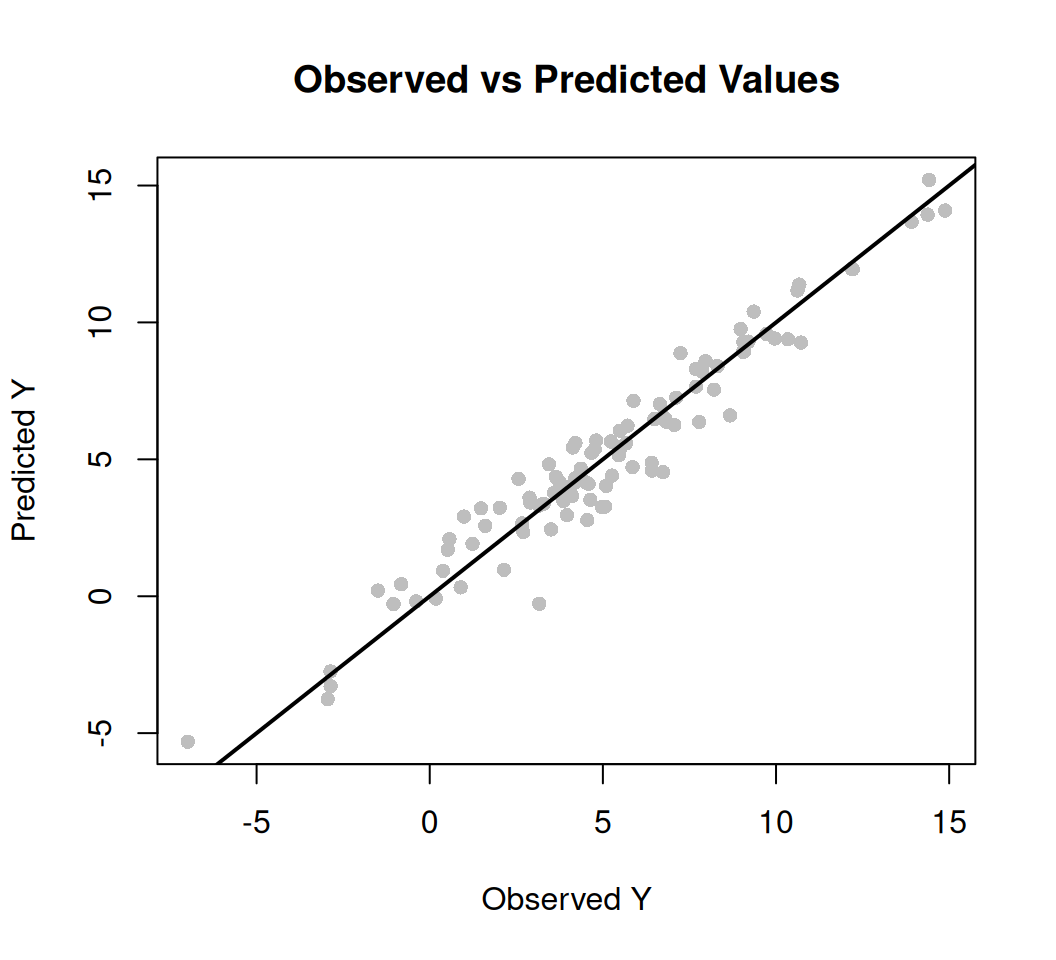
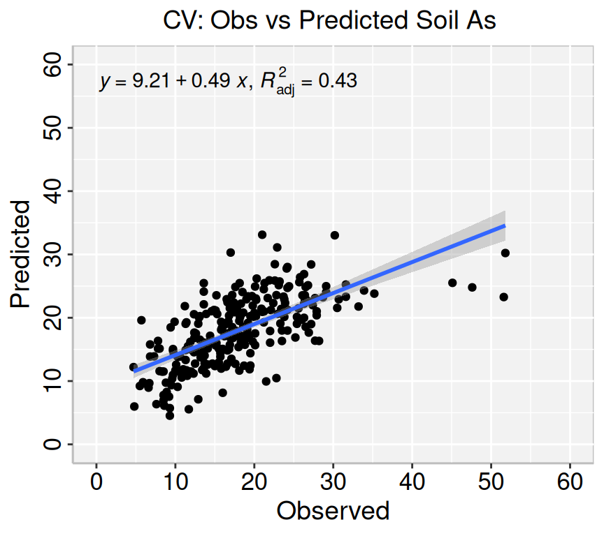
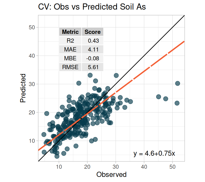
Land_type). The model's explanatory power is substantial (R2 = 0.57). The
model's intercept, corresponding to WAs = 0, WP = 0, WFe = 0, WEc = 0, WpH = 0,
SAoFe = 0, SpH = 0, SOC = 0, SP = 0, Elevation = 0, Year_Irrigation = 0,
Distance_STW = 0, Silt_Sand = 0 and Land_type = HL, is at 13.04 (95% CI [4.64,
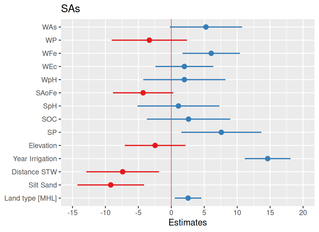
21.45], t(168) = 3.04, p = 0.002). Within this model:

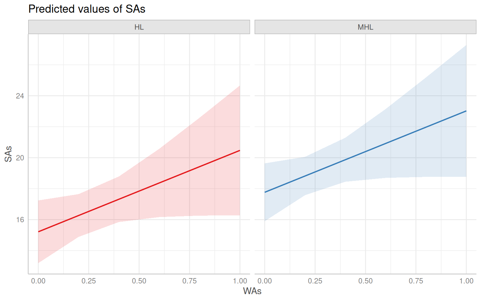
  - The effect of WAs is statistically non-significant and positive (beta = 5.26,
95% CI [-0.23, 10.75], t(168) = 1.88, p = 0.060; Std. beta = 0.13, 95% CI
[-5.70e-03, 0.27])
  - The effect of WP is statistically non-significant and negative (beta = -3.33,
95% CI [-9.05, 2.39], t(168) = -1.14, p = 0.253; Std. beta = -0.07, 95% CI
[-0.19, 0.05])
  - The effect of WFe is statistically significant and positive (beta = 6.06, 95%
CI [1.71, 10.42], t(168) = 2.73, p = 0.006; Std. beta = 0.18, 95% CI [0.05,
0.31])
  - The effect of WEc is statistically non-significant and positive (beta = 1.99,
95% CI [-2.40, 6.38], t(168) = 0.89, p = 0.374; Std. beta = 0.05, 95% CI
[-0.06, 0.16])
  - The effect of WpH is statistically non-significant and positive (beta = 1.98,
95% CI [-4.25, 8.22], t(168) = 0.62, p = 0.533; Std. beta = 0.04, 95% CI
[-0.09, 0.17])
  - The effect of SAoFe is statistically non-significant and negative (beta =
-4.28, 95% CI [-8.85, 0.29], t(168) = -1.83, p = 0.067; Std. beta = -0.10, 95%
CI [-0.21, 6.85e-03])
  - The effect of SpH is statistically non-significant and positive (beta = 1.08,
95% CI [-5.13, 7.30], t(168) = 0.34, p = 0.733; Std. beta = 0.02, 95% CI
[-0.10, 0.14])
  - The effect of SOC is statistically non-significant and positive (beta = 2.61,
95% CI [-3.71, 8.94], t(168) = 0.81, p = 0.418; Std. beta = 0.06, 95% CI
[-0.08, 0.19])
  - The effect of SP is statistically significant and positive (beta = 7.59, 95%
CI [1.52, 13.67], t(168) = 2.45, p = 0.014; Std. beta = 0.13, 95% CI [0.03,
0.24])
  - The effect of Elevation is statistically non-significant and negative (beta =
-2.46, 95% CI [-7.07, 2.15], t(168) = -1.04, p = 0.296; Std. beta = -0.07, 95%
CI [-0.21, 0.06])
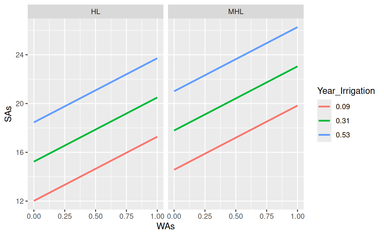
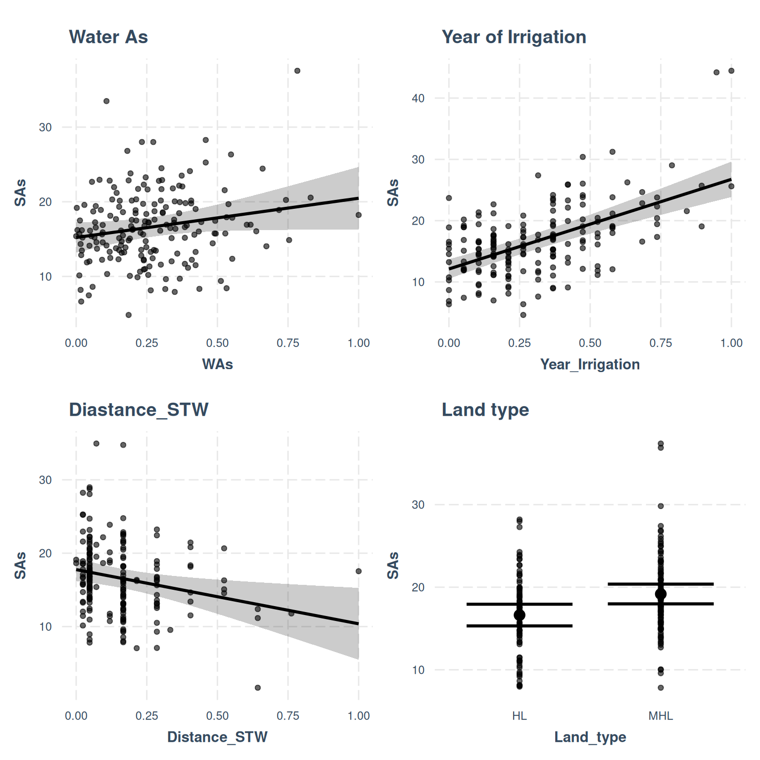
  - The effect of Year Irrigation is statistically significant and positive (beta
= 14.63, 95% CI [11.15, 18.10], t(168) = 8.25, p < .001; Std. beta = 0.44, 95%
CI [0.34, 0.55])
  - The effect of Distance STW is statistically significant and negative (beta =
-7.38, 95% CI [-12.91, -1.86], t(168) = -2.62, p = 0.009; Std. beta = -0.15,
95% CI [-0.27, -0.04])
  - The effect of Silt Sand is statistically significant and negative (beta =
-9.19, 95% CI [-14.24, -4.13], t(168) = -3.56, p < .001; Std. beta = -0.20, 95%
CI [-0.31, -0.09])
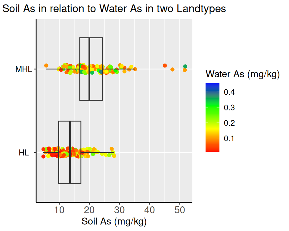
  - The effect of Land type [MHL] is statistically significant and positive (beta
= 2.55, 95% CI [0.53, 4.57], t(168) = 2.47, p = 0.013; Std. beta = 0.35, 95% CI
[0.07, 0.62])

Standardized parameters were obtained by fitting the model on a standardized
version of the dataset. 95% Confidence Intervals (CIs) and p-values were
computed using a Wald t-distribution approximation.

Model Performance

Model performance can be evaluated using model_performance() function of {performance} package.

Code
performance::model_performance(fit.glm)
# Indices of model performance

AIC      |     AICc |      BIC |    R2 |  RMSE | Sigma
------------------------------------------------------
1125.030 | 1128.307 | 1176.381 | 0.569 | 4.795 | 5.004

Visualization of Model Assumptions

The package performance provides many functions to check model assumptions, like check_collinearity(), check_normality() or check_heteroscedasticity(). To get a comprehensive check, use check_model().

Code
performance::check_model(fit.glm)

Marginal Effects and Adjusted Predictions

The presentation of regression models, typically in the form of tables, is widely accepted as a clear and accessible method for interpreting results. However, for more intricate models that incorporate interaction or transformed terms, such as quadratic or spline terms, the use of raw regression coefficients may prove less effective, resulting in challenges when interpreting outcomes. In such cases, adjusted predictions or marginal means provide a more fitting solution. The use of visual aids can also assist in the comprehension of such effects or predictions, providing an intuitive understanding of the relationship between predictors and outcomes, even for complex models.

If we want the marginal effects for “Land_types”, you may use margins() function of {margins} package:

Code
margins::margins(fit.glm, variables = "Land_type")
 Land_typeMHL
        2.551
Note

Marginal Effects: These refer to the change in the dependent variable when an independent variable changes by one unit, while holding all other variables constant. In simpler terms, it tells us the impact of a small change in one variable on another variable, assuming everything else remains unchanged. Marginal effects are often calculated using derivatives in mathematical models. hey are not the same as marginal means or adjusted prediction

we get the same marginal effect using avg_slopes() function from the {marginaleffects} package

Code
marginaleffects::avg_slopes(fit.glm, variables = "Land_type")

 Estimate Std. Error    z Pr(>|z|)   S 2.5 % 97.5 %
     2.55       1.03 2.47   0.0134 6.2 0.529   4.57

Term: Land_type
Type:  response 
Comparison: MHL - HL

ggeffects is a user-friendly package that helps to calculate adjusted predictions, also known as estimated marginal means, with ease. It allows you to calculate these predictions at the mean or representative values of covariates from statistical models. Additionally, you can compare pairwise contrasts, test predictions and differences in predictions for statistical significance, and produce visually appealing figures to display the results.

The package is built around three core functions:

  • predict_response() (understand your results)

  • test_predictions() (check for “significant” results)

  • plot() (communicate your results)

To calculate marginal effects and adjusted predictions, the predict_response() function is used. This function can return three types of predictions, namely, conditional effects, marginal effects or marginal means, and average marginal effects or counterfactual predictions. You can set the type of prediction you want by using the margin argument.

Code
effect<-ggeffects::predict_response(fit.glm, "Land_type", margin = "empirical")
effect
# Average predicted values of SAs

Land_type | Predicted |       95% CI
------------------------------------
HL        |     16.63 | 15.31, 17.94
MHL       |     19.18 | 17.98, 20.37

The marginal effects of “MHL”, relative to “HL” is:

Code
effect$predicted[2] - effect$predicted[1]
[1] 2.551465

{ggeffects} package supports labelled data and the plot() method automatically sets titles, axis - and legend-labels depending on the value and variable labels of the data.

Code
was.landtypes <- ggeffects::predict_response(fit.glm, terms = c("WAs", "Land_type"))
plot(was.landtypes, facets = TRUE)

Code
was.landtypes.year<- ggeffects::predict_response(fit.glm, terms = c("WAs", "Year_Irrigation", "Land_type"))
was.landtypes.year
# Predicted values of SAs

Year_Irrigation: 0.09
Land_type: HL

 WAs | Predicted |       95% CI
-------------------------------
0.00 |     12.02 |  9.95, 14.09
0.20 |     13.07 | 11.59, 14.56
0.60 |     15.18 | 12.86, 17.49
1.00 |     17.28 | 13.00, 21.56

Year_Irrigation: 0.09
Land_type: MHL

 WAs | Predicted |       95% CI
-------------------------------
0.00 |     14.57 | 12.53, 16.61
0.20 |     15.62 | 14.11, 17.14
0.60 |     17.73 | 15.29, 20.16
1.00 |     19.83 | 15.43, 24.23

Year_Irrigation: 0.31
Land_type: HL

 WAs | Predicted |       95% CI
-------------------------------
0.00 |     15.24 | 13.21, 17.26
0.20 |     16.29 | 14.91, 17.67
0.60 |     18.39 | 16.19, 20.60
1.00 |     20.50 | 16.30, 24.69

Year_Irrigation: 0.31
Land_type: MHL

 WAs | Predicted |       95% CI
-------------------------------
0.00 |     17.79 | 15.92, 19.66
0.20 |     18.84 | 17.60, 20.08
0.60 |     20.94 | 18.72, 23.17
1.00 |     23.05 | 18.79, 27.31

Year_Irrigation: 0.53
Land_type: HL

 WAs | Predicted |       95% CI
-------------------------------
0.00 |     18.46 | 16.20, 20.71
0.20 |     19.51 | 17.83, 21.18
0.60 |     21.61 | 19.26, 23.97
1.00 |     23.71 | 19.47, 27.96

Year_Irrigation: 0.53
Land_type: MHL

 WAs | Predicted |       95% CI
-------------------------------
0.00 |     21.01 | 19.00, 23.01
0.20 |     22.06 | 20.66, 23.46
0.60 |     24.16 | 21.89, 26.43
1.00 |     26.27 | 22.01, 30.52

Adjusted for:
*           WP = 0.36
*          WFe = 0.40
*          WEc = 0.24
*          WpH = 0.44
*        SAoFe = 0.40
*          SpH = 0.73
*          SOC = 0.39
*           SP = 0.27
*    Elevation = 0.41
* Distance_STW = 0.15
*    Silt_Sand = 0.53
Code
# select specific levels for grouping terms
ggplot(was.landtypes.year, aes(x = x, y = predicted, colour = group)) +
  stat_smooth(method = "lm", se = FALSE) +
  facet_wrap(~facet) +
  labs(
    y = ggeffects::get_y_title(was.landtypes.year),
    x = ggeffects::get_x_title(was.landtypes.year),
    colour = ggeffects::get_legend_title(was.landtypes.year)
  )

effect_plot() function of {jtools} package also plot simple effects in GLM regression models:

Code
p1<-jtools::effect_plot(fit.glm, 
                    main.title = "Water As", 
                    pred = WAs, 
                    interval = TRUE,  
                    partial.residuals = TRUE)
p2<-jtools::effect_plot(fit.glm, 
                    main.title = "Year of Irrigation ", 
                    pred = Year_Irrigation, 
                    interval = TRUE,  
                    partial.residuals = TRUE)
p3<-jtools::effect_plot(fit.glm, 
                    main.title = "Diastance_STW", 
                    pred = Distance_STW , 
                    interval = TRUE,  
                    partial.residuals = TRUE)
p4<-jtools::effect_plot(fit.glm, 
                    main.title = "Land type", 
                    pred = Land_type, 
                    interval = TRUE,  
                    partial.residuals = TRUE)
library(patchwork)
(p1+p2)/(p3 +p4)

Cross-validation

k-fold Cross-validation

The {boot} package’s cv.glm() function provides an easy way to do k-fold cross-validation on GLM models. Here first we fit GLM model for entire dataset then we apply cv.glm() on fitted glm object.

Code
fit.glm.mf<-glm(SAs~.,mf, 
             family= gaussian(link = "identity")
             )  
cv_result <- cv.glm(data = mf, glmfit = fit.glm.mf, K = 5)

# Print cross-validation error
print(cv_result$delta)
[1] 7.870229 7.648387

However, this cv.glm() function does not directly provide predicted values for each observation in the test folds; it only provides the cross-validated error estimates. However, we can achieve this by manually implementing k-fold cross-validation and storing the predictions for each fold.

Here below you how to implement K-fold cross-validation using the glm() function in R:

Code
# Function for K-fold Cross-Validation with GLM
k_fold_cv_glm <- function(data, formula, k = 5) {
  # Check that the number of folds is valid
  if (k <= 1 || k > nrow(data)) {
    stop("Invalid number of folds.")
  }
  
  # Create a vector to store mean squared errors for each fold
  cv_mse <- numeric(k)  
  # Vector to store predicted values
  predicted_values <- numeric(nrow(data))
  
  # Randomly assign folds
  set.seed(42)  # Ensure reproducibility
  folds <- sample(1:k, nrow(data), replace = TRUE)

  # K-fold Cross-validation Loop
  for (fold in 1:k) {
    # Create training and test sets
    test_idx <- which(folds == fold)  # Test indices for current fold
    train_idx <- setdiff(1:nrow(data), test_idx)  # Train indices

    # Create training and test datasets
    train_data <- data[train_idx, ]
    test_data <- data[test_idx, ]

    # Fit the GLM model on the training set
    model <- glm(formula, data = train_data)

    # Predict on the test set
    Y_pred <- predict(model, newdata = test_data)

    # Store predicted values for the current fold
    predicted_values[test_idx] <- Y_pred

    # Calculate Mean Squared Error (MSE) for this fold
    cv_mse[fold] <- mean((test_data[[as.character(formula[[2]])]] - Y_pred)^2)
  }

  # Return the average MSE and the predicted values
  return(list(average_mse = mean(cv_mse), predicted_values = predicted_values))
}

formula = SAs ~ WAs + WP + WFe + WEc + WpH + SAoFe + SpH + SOC +
                Sand + Silt+ SP + Elevation +
                Year_Irrigation + Distance_STW +
                Land_type

cv.glm <- k_fold_cv_glm(mf, formula, k = 5)  # Run K-fold CV

# Display Average Cross-Validation MSE
cat("Average Cross-Validation MSE:", cv.glm$average_mse, "\n")
Average Cross-Validation MSE: 31.70601 
Code
# Step 4: Compare Predicted vs Observed Values
mf$Pred.SAs <- cv.glm$predicted_values

CV Prediction Performance

The {Matrics} package offers several useful functions to evaluate the performance of a regression model.

Code
RMSE<- Metrics::rmse(mf$SAs, mf$Pred.SAs)
MAE<- Metrics::mae(mf$SAs, mf$Pred.SAs)
MSE<- Metrics::mse(mf$SAs, mf$Pred.SAs)
MDAE<- Metrics::mdae(mf$SAs, mf$Pred.SAs)
print(peformance.matrics<-cbind("RMSE"=RMSE,
                                "MAE" = MAE, 
                                "MSE" = MSE, 
                                "MDAE" = MDAE))
         RMSE      MAE      MSE     MDAE
[1,] 5.613283 4.106696 31.50895 3.276106

metrics_summary() function of {metrica} package estimates a group of metrics characterizing the prediction performance of the model:

Code
my.metrics <- c("R2","RMSE", "MAE", "MBE")

metrics_summary(data = mf,   
                obs = SAs,    
                pred = Pred.SAs,
                type = "regression",
                metrics_list = my.metrics
                 )                
  Metric       Score
1     R2  0.42913604
2    MAE  4.10669598
3    MBE -0.08211394
4   RMSE  5.61328325

1:1 Plot

We can plot observed and predicted values with fitted regression line with {ggplot2} and {ggpmisc} packages.

Code
library(ggpmisc)
formula<-y~x

ggplot(mf, aes(SAs,Pred.SAs)) +
  geom_point() +
  geom_smooth(method = "lm")+
  stat_poly_eq(use_label(c("eq", "adj.R2")), formula = formula) +
  ggtitle("CV: Obs vs Predicted Soil As ") +
  xlab("Observed") + ylab("Predicted") +
  scale_x_continuous(limits=c(0,60), breaks=seq(0, 60, 10))+ 
  scale_y_continuous(limits=c(0,60), breaks=seq(0, 60, 10)) +
  # Flip the bars
  theme(
    panel.background = element_rect(fill = "grey95",colour = "gray75",size = 0.5, linetype = "solid"),
    axis.line = element_line(colour = "grey"),
    plot.title = element_text(size = 14, hjust = 0.5),
    axis.title.x = element_text(size = 14),
    axis.title.y = element_text(size = 14),
    axis.text.x=element_text(size=13, colour="black"),
    axis.text.y=element_text(size=13,angle = 90,vjust = 0.5, hjust=0.5, colour='black'))

scatter_plot() function of {metrica} draws a scatter plot of predictions and observations with alternative axis orientation. To print the metrics on the scatter_plot(), just use print.metrics =TRUE.

Code
my.metrica.plot <- scatter_plot(data = mf,
                obs = SAs,    
                pred = Pred.SAs,
                print_metrics = TRUE, 
                metrics_list = my.metrics,
                 position_metrics = c(x = 10, y = 50)) +
                 ggtitle("CV: Obs vs Predicted Soil As ") +
                theme_light()
my.metrica.plot

Prediction at Test Locations

The predict() function will be used to predict the amount of SOC present in the testing locations. This will help to validate the accuracy of the GLM regression model.

Code
test$Pred.SAs<-predict(fit.glm, test)  

Prediction Performance

The {Matrics} package offers several useful functions to evaluate the performance of a regression model.

Code
RMSE<- Metrics::rmse(test$SAs, test$Pred.SAs)
MAE<- Metrics::mae(test$SAs, test$Pred.SAs)
MSE<- Metrics::mse(test$SAs, test$Pred.SAs)
MDAE<- Metrics::mdae(test$SAs, test$Pred.SAs)
print(peformance.matrics<-cbind("RMSE"=RMSE,
                                "MAE" = MAE, 
                                "MSE" = MSE, 
                                "MDAE" = MDAE))
         RMSE      MAE      MSE     MDAE
[1,] 5.765459 3.892464 33.24052 2.543197

1:1 Plot

We can plot observed and predicted values with fitted regression line with {ggplot2} and {ggpmisc} packages.

Code
library(ggpmisc)
formula<-y~x

ggplot(test, aes(SAs,Pred.SAs)) +
  geom_point() +
  geom_smooth(method = "lm")+
  stat_poly_eq(use_label(c("eq", "adj.R2")), formula = formula) +
  ggtitle("Test data: Obs vs Predicted Soil As ") +
  xlab("Observed") + ylab("Predicted") +
  scale_x_continuous(limits=c(0,60), breaks=seq(0, 60, 10))+ 
  scale_y_continuous(limits=c(0,60), breaks=seq(0, 60, 10)) +
  # Flip the bars
  theme(
    panel.background = element_rect(fill = "grey95",colour = "gray75",size = 0.5, linetype = "solid"),
    axis.line = element_line(colour = "grey"),
    plot.title = element_text(size = 14, hjust = 0.5),
    axis.title.x = element_text(size = 14),
    axis.title.y = element_text(size = 14),
    axis.text.x=element_text(size=13, colour="black"),
    axis.text.y=element_text(size=13,angle = 90,vjust = 0.5, hjust=0.5, colour='black'))

scatter_plot() function of {metrica} draws a scatter plot of predictions and observations with alternative axis orientation. To print the metrics on the scatter_plot(), just use print.metrics =TRUE.

Code
test.metrica.plot <- scatter_plot(data = test,
                obs = SAs,    
                pred = Pred.SAs,
                print_metrics = TRUE, 
                metrics_list = my.metrics,
                 position_metrics = c(x = 10, y = 50)) +
                 ggtitle("Test Data: Obs vs Predicted Soil As ") +
                theme_light()
test.metrica.plot

Summary and Conclusion

This comprehensive tutorial covered the essentials of conducting Generalized Linear Model (GLM) regression analysis with a Gaussian distribution in R, from foundational concepts to advanced interpretation and evaluation techniques. We began by introducing the structure and key components of GLMs, particularly those that use the Gaussian distribution, and explored their suitability for continuous data. Building a GLM model from scratch allowed us to understand the model’s structure, including the linear predictors, error terms, and link functions.

Next, we used R’s glm() function to fit a Gaussian GLM more efficiently and compared it with the simpler lm() function, which directly applies to linear models. The tutorial guided interpreting model outputs, including understanding coefficients, statistical significance, and key model metrics. For this, we leveraged a range of powerful R packages such as {performance}, {report}, {ggeffects}, and {jtools} to streamline and enhance our interpretation and visualization of GLM outputs, making it easier to extract meaningful insights from the model. We then addressed model performance evaluation using cross-validation and a hold-out test data set, demonstrating how these methods help assess model generalization and prevent overfitting. By using cross-validation and a separate test data set, we ensured a robust and unbiased estimate of model performance, essential for applying the model confidently to new data.

This tutorial equipped you with a thorough understanding of Gaussian GLMs, from constructing models and using R’s built-in functions to interpreting results and evaluating model performance. With knowledge of theoretical underpinnings and practical tools, you are now well-prepared to perform GLM regression analysis in R. The tutorial highlighted various packages that simplify and enhance interpretation, allowing you to select the tools that best align with your analytically goals—whether prioritizing simplicity, flexibility, or advanced customization. Armed with this knowledge, you can confidently apply GLM regression techniques to analyze continuous data in diverse fields and effectively communicate your findings through clear interpretations and visuals, making GLMs an invaluable tool in your data analysis toolkit.

References

  1. 6.1 - Introduction to GLMs

  2. GLM in R: Generalized Linear Model

  3. GLM in R: Generalized Linear Model with Example

  4. Generalized Linear Models With Examples in R

Session Info

Code
sessionInfo()
R version 4.4.2 (2024-10-31)
Platform: x86_64-pc-linux-gnu
Running under: Ubuntu 24.04.1 LTS

Matrix products: default
BLAS:   /usr/lib/x86_64-linux-gnu/blas/libblas.so.3.12.0 
LAPACK: /usr/lib/x86_64-linux-gnu/lapack/liblapack.so.3.12.0

locale:
 [1] LC_CTYPE=en_US.UTF-8       LC_NUMERIC=C              
 [3] LC_TIME=en_US.UTF-8        LC_COLLATE=en_US.UTF-8    
 [5] LC_MONETARY=en_US.UTF-8    LC_MESSAGES=en_US.UTF-8   
 [7] LC_PAPER=en_US.UTF-8       LC_NAME=C                 
 [9] LC_ADDRESS=C               LC_TELEPHONE=C            
[11] LC_MEASUREMENT=en_US.UTF-8 LC_IDENTIFICATION=C       

time zone: America/New_York
tzcode source: system (glibc)

attached base packages:
[1] stats     graphics  grDevices utils     datasets  methods   base     

other attached packages:
 [1] metrica_2.1.0          Metrics_0.1.4          report_0.6.1          
 [4] jtools_2.3.0           gtsummary_2.1.0        gt_0.11.1             
 [7] patchwork_1.3.0        sjPlot_2.8.17          ggpmisc_0.6.1         
[10] ggpp_0.5.8-1           performance_0.13.0     ggeffects_2.2.0       
[13] marginaleffects_0.25.0 margins_0.3.28         boot_1.3-31           
[16] rstatix_0.7.2          plyr_1.8.9             lubridate_1.9.4       
[19] forcats_1.0.0          stringr_1.5.1          dplyr_1.1.4           
[22] purrr_1.0.4            readr_2.1.5            tidyr_1.3.1           
[25] tibble_3.2.1           ggplot2_3.5.1          tidyverse_2.0.0       

loaded via a namespace (and not attached):
  [1] RColorBrewer_1.1-3   rstudioapi_0.17.1    jsonlite_1.9.0      
  [4] datawizard_1.0.2     magrittr_2.0.3       TH.data_1.1-3       
  [7] estimability_1.5.1   farver_2.1.2         rmarkdown_2.29      
 [10] minerva_1.5.10       vctrs_0.6.5          memoise_2.0.1       
 [13] base64enc_0.1-3      effectsize_1.0.0     htmltools_0.5.8.1   
 [16] energy_1.7-12        polynom_1.4-1        curl_6.2.1          
 [19] haven_2.5.4          broom_1.0.7          Formula_1.2-5       
 [22] sjmisc_2.8.10        sass_0.4.9           parallelly_1.42.0   
 [25] htmlwidgets_1.6.4    sandwich_3.1-1       emmeans_1.11.0      
 [28] zoo_1.8-13           cachem_1.1.0         commonmark_1.9.2    
 [31] lifecycle_1.0.4      pkgconfig_2.0.3      sjlabelled_1.2.0    
 [34] Matrix_1.7-1         R6_2.6.1             fastmap_1.2.0       
 [37] future_1.34.0        digest_0.6.37        colorspace_2.1-1    
 [40] furrr_0.3.1          confintr_1.0.2       RSQLite_2.3.9       
 [43] labeling_0.4.3       timechange_0.3.0     mgcv_1.9-1          
 [46] abind_1.4-8          compiler_4.4.2       bit64_4.6.0-1       
 [49] withr_3.0.2          pander_0.6.5         gsl_2.1-8           
 [52] backports_1.5.0      carData_3.0-5        DBI_1.2.3           
 [55] prediction_0.3.18    broom.mixed_0.2.9.6  MASS_7.3-64         
 [58] quantreg_6.1         sjstats_0.19.0       tools_4.4.2         
 [61] glue_1.8.0           nlme_3.1-166         grid_4.4.2          
 [64] checkmate_2.3.2      see_0.11.0           generics_0.1.3      
 [67] gtable_0.3.6         labelled_2.14.0      tzdb_0.4.0          
 [70] data.table_1.17.0    hms_1.1.3            xml2_1.3.6          
 [73] car_3.1-3            utf8_1.2.4           ggrepel_0.9.6       
 [76] pillar_1.10.1        markdown_1.13        vroom_1.6.5         
 [79] splines_4.4.2        lattice_0.22-5       survival_3.8-3      
 [82] bit_4.5.0.1          SparseM_1.84-2       tidyselect_1.2.1    
 [85] knitr_1.49           gridExtra_2.3        svglite_2.1.3       
 [88] xfun_0.51            stringi_1.8.4        yaml_2.3.10         
 [91] kableExtra_1.4.0     evaluate_1.0.3       codetools_0.2-20    
 [94] cli_3.6.4            systemfonts_1.2.1    xtable_1.8-4        
 [97] parameters_0.24.2    munsell_0.5.1        Rcpp_1.0.14         
[100] globals_0.16.3       coda_0.19-4.1        parallel_4.4.2      
[103] MatrixModels_0.5-3   blob_1.2.4           bayestestR_0.15.2   
[106] listenv_0.9.1        viridisLite_0.4.2    broom.helpers_1.20.0
[109] mvtnorm_1.3-3        scales_1.3.0         insight_1.1.0       
[112] crayon_1.5.3         rlang_1.1.5          multcomp_1.4-28     
[115] cards_0.5.0.9000