6. Joint Modeling of Longitudinal and Time-to-Event Data

Joint models offer a powerful framework for analyzing complex clinical datasets and generating accurate predictions for longitudinal and survival outcomes. By integrating longitudinal and time-to-event data, joint models provide a holistic view of disease progression and patient outcomes, enabling researchers to make informed decisions and improve patient care. In this chapter, we introduce the concept of joint modeling, discuss its advantages, and demonstrate how to fit joint models in R using the {JM}, {JMbayes2} and {joineR} packages. We provide examples of joint models for longitudinal and time-to-event data, including model fitting, prediction, and interpretation. By the end of this chapter, you will have a solid understanding of joint modeling and be able to apply it to your own research projects.

Overview

Longitudinal and Time-to-Event data

Longitudinal and Time-to-Event data are commonly encountered in studies involving repeated measurements and event tracking over Time. Understanding these data types is essential for developing statistical models, particularly joint models.

Longitudinal data consist of repeated observations of the same variable(s) over Time for each individual or unit of observation. These data capture the trajectory or progression of a response variable within subjects over Time. The most common examples of longitudinal data are tracking patients’ blood pressure every month for a year, and monitoring students’ test scores over several semesters.

Key features of longitudinal data: - Repeated Measurements: Data are collected at multiple time points for each subject. - Time-Dependent Trends: The focus is often on how the response variable changes over Time. - Correlated Observations: Measurements within the same individual are typically correlated.

Time-to-event data (also known as survival data) involves measuring the Time until an event of interest occurs. The event could be anything, such as death, disease onset, system failure, or recovery. Time from cancer diagnosis to death and until a machine breaks down are examples of Time-to-event data.

Key features of Time-to-event data:

  • Event of Interest: The focus is on the occurrence of a specific event.
  • Censoring: Some subjects may not experience the event during the study period, and their time-to-event is only partially known (e.g., right-censoring when the study ends before the event occurs).
  • Non-Normality: Time-to-event data are often skewed and require specialized modeling techniques like Kaplan-Meier estimation or Cox proportional hazards models.

Combining Longitudinal and Time-to-Event Data

In many studies, longitudinal and time-to-event data are collected together. For example:

  • Clinical Trials: Repeated measures of a biomarker (e.g., cholesterol levels) and the Time until a heart attack.

  • Chronic Disease Studies: Disease progression (e.g., lung function decline) and survival time.

Joint Modeling of Longitudinal and Time-to-Event Data*

Joint Modeling of Longitudinal and Time-to-Event Data is a statistical approach designed to simultaneously analyze longitudinal (repeated measures) and time-to-event (survival) data, especially when these two types of data are correlated. The methodology links the two processes, enabling a more accurate understanding of their relationship and better predictions of outcomes.

Why Use Joint Models?

  1. Dependency Between Data Types:
    • Longitudinal markers (e.g., biomarkers, repeated measurements) often influence or are associated with survival outcomes. Ignoring this dependency can lead to biased results.
    • For example, in a cancer study, a biomarker like PSA (prostate-specific antigen) measured over time can be predictive of time to disease progression or death.
  2. Separate Models are Insufficient:
    • Longitudinal models (e.g., linear mixed models) focus only on repeated measurements and ignore survival times.
    • Survival models (e.g., Cox proportional hazards) treat longitudinal measures as static covariates, losing information about their dynamic nature.
  3. Prediction:
    • Joint models allow dynamic predictions of survival probabilities based on the evolving trajectory of the longitudinal marker.

Structure of Joint Models

A joint model consists of two submodels that are linked by a shared structure:

1. Longitudinal Submodel

  • Models the repeated measurements of the longitudinal outcome over time.
  • Example: A linear mixed-effects model (LMM):

\[ y_i(t) = X_i(t)\beta + Z_i(t)b_i + \epsilon_i(t), \] where:

  • \(y_i(t)\): Longitudinal outcome for subject \(i\) at time \(t\).
  • \(X_i(t)\): Fixed-effects covariates with coefficients \(\beta\).
  • \(Z_i(t)b_i\): Random effects capturing individual-specific deviations.
  • \(\epsilon_i(t)\): Measurement error.

2. Survival Submodel

  • Models the time-to-event data, incorporating information from the longitudinal submodel.
  • Example: A proportional hazards model:

\[ h_i(t) = h_0(t) \exp\{W_i\gamma + \alpha m_i(t)\} \]

where:

  • \(h_i(t)\): Hazard function for subject \(i\) at time \(t\).
  • \(h_0(t)\): Baseline hazard.
  • \(W_i\gamma\): Covariate effects on survival.
  • \(m_i(t)\): Longitudinal marker at time \(t\).
  • \(\alpha\): Association parameter linking longitudinal and survival submodels.

3. Association Structure

  • Defines how the longitudinal marker influences the survival process. Common forms include:

    • Current Value: Survival depends on the marker’s value at time \(t\).
    • Slope: Survival depends on the rate of change of the marker.
    • Cumulative Effect: Survival depends on the marker’s trajectory over time (e.g., area under the curve).

Advantages of Joint Models

  1. Bias Reduction:
    • Accounts for the measurement error in longitudinal data when used as a predictor in survival models.
  2. Improved Efficiency:
    • Utilizes all available data simultaneously, leading to more precise estimates.
  3. Dynamic Prediction:
    • Enables real-time updating of survival probabilities based on the latest longitudinal information.

Applications

  1. Medicine:
    • Monitoring disease biomarkers (e.g., tumor size, glucose levels) and predicting survival outcomes.
  2. Drug Development:
    • Understanding the relationship between pharmacokinetics/pharmacodynamics and patient outcomes.
  3. Engineering:
    • Modeling degradation of machinery (longitudinal) and time to failure (event data).

Example

Consider a study where patients’ kidney function (measured by glomerular filtration rate, GFR) is monitored over time, and the time to kidney failure is recorded.

  1. Longitudinal Submodel:

    • Captures the decline in GFR over time, accounting for patient-specific variability.
  2. Survival Submodel:

    • Models the hazard of kidney failure, influenced by the current GFR levels.
  3. Joint Model:

    • Links the two submodels, providing insights into how declining GFR predicts the risk of kidney failure.

Joint Modeling of Longitudinal and Time-to-Event Data in R

Joint modeling of longitudinal and time-to-event data in R can be efficiently performed using several packages like {JM}, {joineR}, and {joineRML}. These packages provide tools for estimating parameters and making predictions for both submodels simultaneously. Below, we outline the process and examples using {JM} and {JMbayes}, two widely used packages.

Install Required R Packages

Following R packages are required to run this notebook. If any of these packages are not installed, you can install them using the code below:

Code
packages <-c(
         'tidyverse',
         'survival',
         'survminer',
         'ggsurvfit',
         'tidycmprsk',
         'ggfortify',
         'timereg',
         'cmprsk',
         'condSURV',
         'riskRegression',
         'prodlim',
         'lava',
         'mstate',
         'regplot',
         'cmprskcoxmsm',
         'GLMMadaptive',
         'JM',
         'nlme',
         'lattice',
         'joineR',
         'joineRML'
         
         )
#| warning: false
#| error: false

# Install missing packages
new_packages <- packages[!(packages %in% installed.packages()[,"Package"])]
if(length(new_packages)) install.packages(new_packages)

devtools::install_github("ItziarI/WeDiBaDis")

# Verify installation
cat("Installed packages:\n")
print(sapply(packages, requireNamespace, quietly = TRUE))

Load Packages

Code
# Load packages with suppressed messages
invisible(lapply(packages, function(pkg) {
  suppressPackageStartupMessages(library(pkg, character.only = TRUE))
}))
Code
# Check loaded packages
cat("Successfully loaded packages:\n")
Successfully loaded packages:
Code
print(search()[grepl("package:", search())])
 [1] "package:joineRML"       "package:joineR"         "package:lattice"       
 [4] "package:JM"             "package:splines"        "package:nlme"          
 [7] "package:MASS"           "package:GLMMadaptive"   "package:cmprskcoxmsm"  
[10] "package:regplot"        "package:mstate"         "package:lava"          
[13] "package:prodlim"        "package:riskRegression" "package:condSURV"      
[16] "package:cmprsk"         "package:timereg"        "package:ggfortify"     
[19] "package:tidycmprsk"     "package:ggsurvfit"      "package:survminer"     
[22] "package:ggpubr"         "package:survival"       "package:lubridate"     
[25] "package:forcats"        "package:stringr"        "package:dplyr"         
[28] "package:purrr"          "package:readr"          "package:tidyr"         
[31] "package:tibble"         "package:ggplot2"        "package:tidyverse"     
[34] "package:stats"          "package:graphics"       "package:grDevices"     
[37] "package:utils"          "package:datasets"       "package:methods"       
[40] "package:base"          

The {JM} Package

The {JM} package is a comprehensive tool for fitting joint models of longitudinal and time-to-event data in R. It provides functions for estimating the parameters of the longitudinal and survival submodels, as well as the association structure linking the two. The package also offers tools for making predictions and assessing the model’s performance. Below, we demonstrate how to use the {JM} package to fit joint models to longitudinal and time-to-event data.

The joint model consists of two submodels: a linear mixed model for the longitudinal CD4 cell counts and a Cox proportional hazards model for the survival outcomes. The two submodels are linked by a shared parameter that captures the association between the longitudinal and survival processes.

Data

We’ll use the aids dataset from the {JM} package to demonstrate how to perform joint modeling of longitudinal and time-to-event data in R. A randomized clinical trial in which both longitudinal and survival data were collected to compare the efficacy and safety of two antiretroviral drugs in treating patients who had failed or were intolerant of zidovudine (AZT) therapy. The dataset contains information on patients’ CD4 cell counts (CD4) and survival status (death) over time, along with other covariates. The goal is to model the relationship between CD4 cell counts and survival outcomes.

The dataset used is the same that the one seen with the mixed model, aids. The survival information can be found in aids.id.

A data frame with 1408 observations on the following 9 variables.

patiet: patients identifier; in total there are 467 patients.

Time: the time to death or censoring.

death: a numeric vector with 0 denoting censoring and 1 death.

CD4: the CD4 cells count.

obstime: the time points at which the CD4 cells count was recorded.

drug: a factor with levels ddC denoting zalcitabine and ddI denoting didanosine.

gender: a factor with levels female and male.

prevOI: a factor with levels AIDS denoting previous opportunistic infection (AIDS diagnosis) at study entry, and noAIDS denoting no previous infection.

AZT: a factor with levels intolerance and failure denoting AZT intolerance and AZT failure, respectively.

Code
data("aids", package = "JM")
glimpse(aids)
Rows: 1,405
Columns: 12
$ patient <fct> 1, 1, 1, 2, 2, 2, 2, 3, 3, 3, 4, 4, 4, 4, 5, 5, 5, 5, 6, 7, 7,…
$ Time    <dbl> 16.97, 16.97, 16.97, 19.00, 19.00, 19.00, 19.00, 18.53, 18.53,…
$ death   <int> 0, 0, 0, 0, 0, 0, 0, 1, 1, 1, 0, 0, 0, 0, 0, 0, 0, 0, 1, 0, 0,…
$ CD4     <dbl> 10.677078, 8.426150, 9.433981, 6.324555, 8.124038, 4.582576, 5…
$ obstime <int> 0, 6, 12, 0, 6, 12, 18, 0, 2, 6, 0, 2, 6, 12, 0, 2, 6, 12, 0, …
$ drug    <fct> ddC, ddC, ddC, ddI, ddI, ddI, ddI, ddI, ddI, ddI, ddC, ddC, dd…
$ gender  <fct> male, male, male, male, male, male, male, female, female, fema…
$ prevOI  <fct> AIDS, AIDS, AIDS, noAIDS, noAIDS, noAIDS, noAIDS, AIDS, AIDS, …
$ AZT     <fct> intolerance, intolerance, intolerance, intolerance, intoleranc…
$ start   <int> 0, 6, 12, 0, 6, 12, 18, 0, 2, 6, 0, 2, 6, 12, 0, 2, 6, 12, 0, …
$ stop    <dbl> 6.00, 12.00, 16.97, 6.00, 12.00, 18.00, 19.00, 2.00, 6.00, 18.…
$ event   <dbl> 0, 0, 0, 0, 0, 0, 0, 0, 0, 1, 0, 0, 0, 0, 0, 0, 0, 0, 1, 0, 0,…
Code
data("aids.id", package = "JM")
glimpse(aids.id)
Rows: 467
Columns: 12
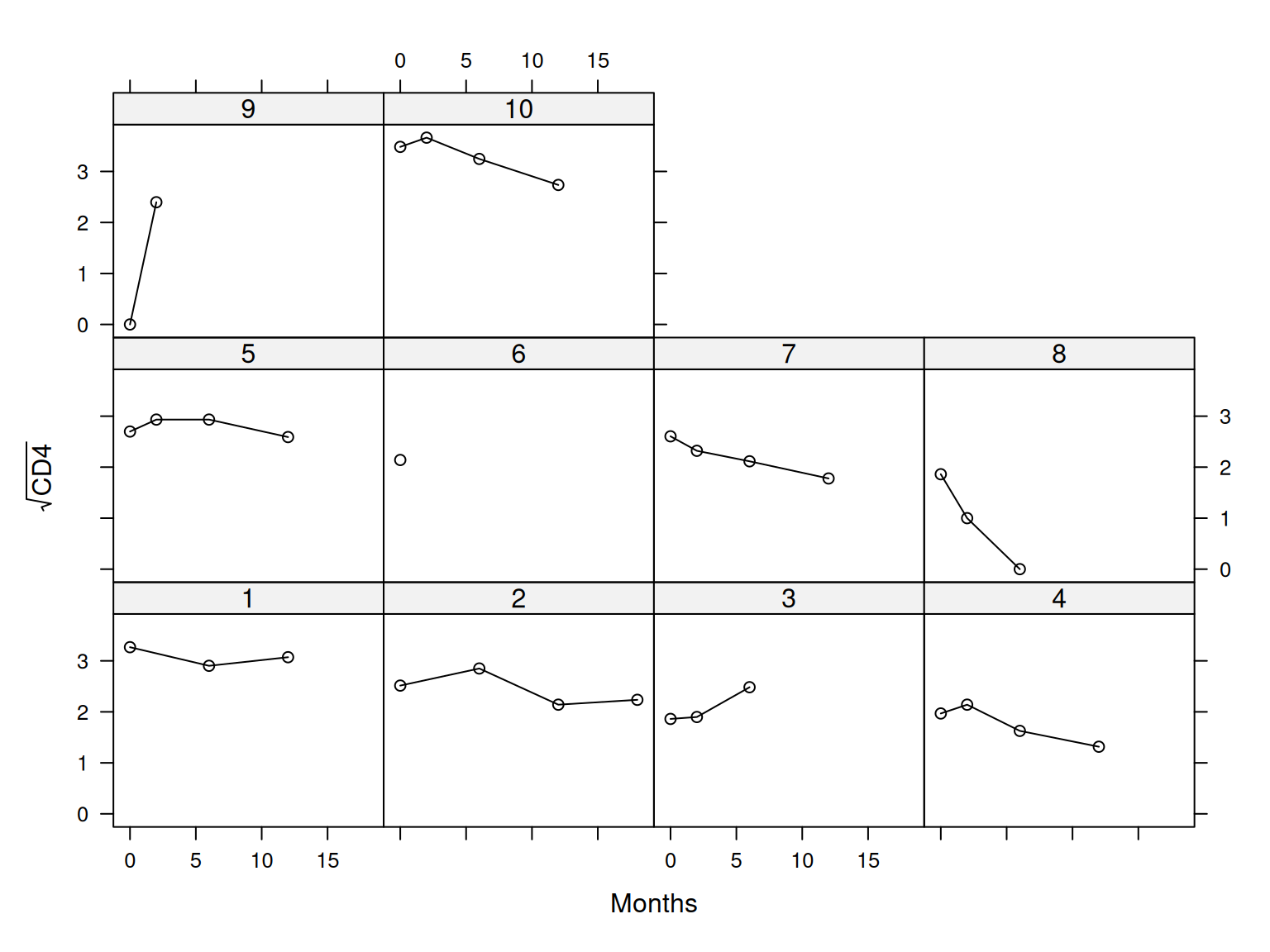
$ patient <fct> 1, 2, 3, 4, 5, 6, 7, 8, 9, 10, 11, 12, 13, 14, 15, 16, 17, 18,…
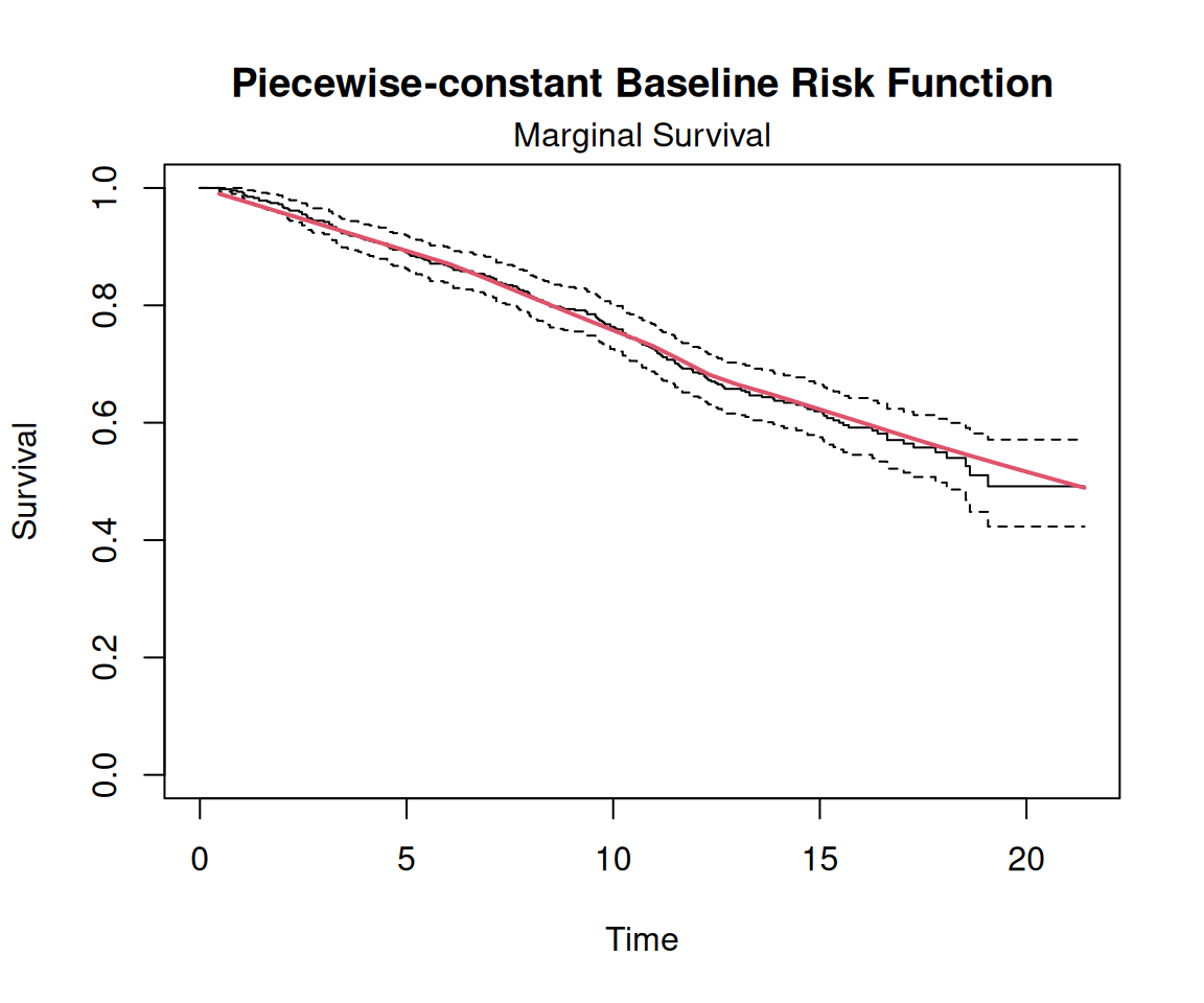
$ Time    <dbl> 16.97, 19.00, 18.53, 12.70, 15.13, 1.90, 14.33, 9.57, 11.57, 1…
$ death   <int> 0, 0, 1, 0, 0, 1, 0, 1, 1, 0, 1, 0, 1, 1, 0, 1, 0, 0, 1, 0, 1,…
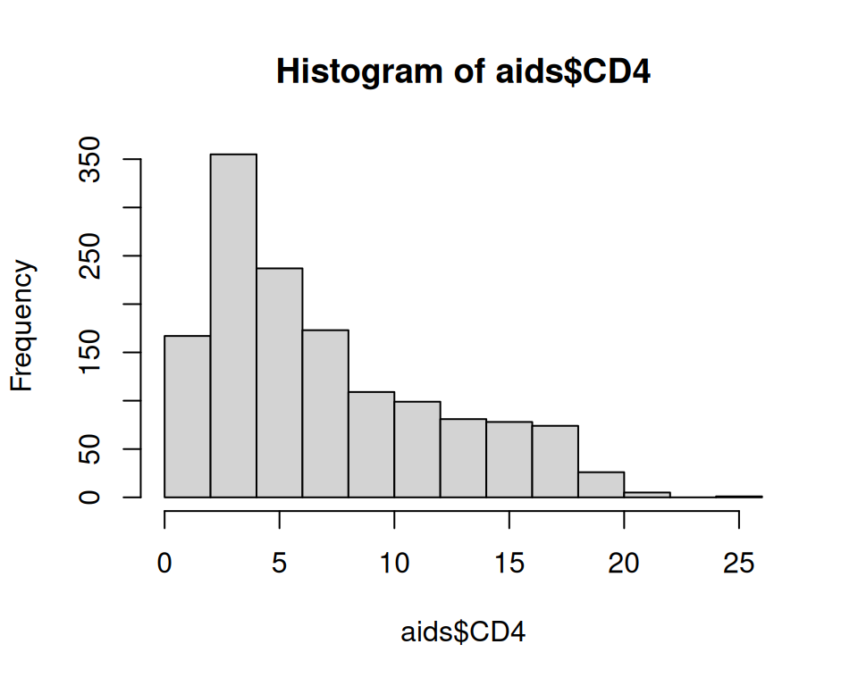
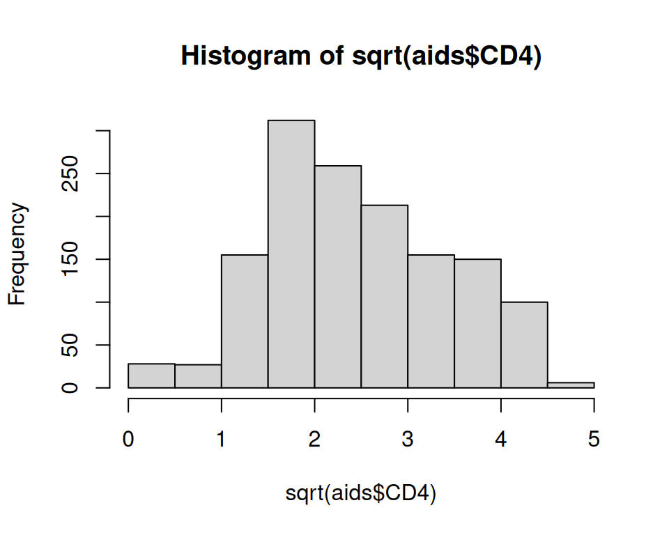
$ CD4     <dbl> 10.677078, 6.324555, 3.464102, 3.872983, 7.280110, 4.582576, 6…
$ obstime <int> 0, 0, 0, 0, 0, 0, 0, 0, 0, 0, 0, 0, 0, 0, 0, 0, 0, 0, 0, 0, 0,…
$ drug    <fct> ddC, ddI, ddI, ddC, ddI, ddC, ddC, ddI, ddC, ddI, ddC, ddI, dd…
$ gender  <fct> male, male, female, male, male, female, male, female, male, ma…
$ prevOI  <fct> AIDS, noAIDS, AIDS, AIDS, AIDS, AIDS, AIDS, noAIDS, AIDS, AIDS…
$ AZT     <fct> intolerance, intolerance, intolerance, failure, failure, failu…
$ start   <int> 0, 0, 0, 0, 0, 0, 0, 0, 0, 0, 0, 0, 0, 0, 0, 0, 0, 0, 0, 0, 0,…
$ stop    <dbl> 6.00, 6.00, 2.00, 2.00, 2.00, 1.90, 2.00, 2.00, 2.00, 2.00, 2.…
$ event   <dbl> 0, 0, 0, 0, 0, 1, 0, 0, 0, 0, 1, 0, 0, 0, 0, 0, 0, 0, 1, 0, 0,…
Code
hist(aids$CD4)

The CD4 cell exhibits right skewed shapes of distribution, and therefore, for the remainder of this analysis we will work with the square root of the CD4 cell values

Code
hist(sqrt(aids$CD4))

Code
lattice::xyplot(sqrt(CD4) ~ obstime | patient, group = patient, 
       data = aids[aids$patient %in% c(1:10),], 
       xlab = "Months", ylab = expression(sqrt("CD4")), col = 1, type = "b")

Fit a Longitudinal Model (lmeObject)

First, we fit a linear mixed model for the longitudinal CD4 cell counts using the lme() function from the {nlme} package. This model captures the trajectory of CD4 cell counts over time, accounting for patient-specific variability.

Code
# linear mixed model fit (random intercepts)
lmeFit_01 <- lme(sqrt(CD4) ~ obstime : drug, random = ~ 1 | patient, data = aids)
summary(lmeFit_01)
Linear mixed-effects model fit by REML
  Data: aids 
       AIC      BIC    logLik
  2730.729 2756.957 -1360.364

Random effects:
 Formula: ~1 | patient
        (Intercept)  Residual
StdDev:   0.8719493 0.4106749

Fixed effects:  sqrt(CD4) ~ obstime:drug 
                     Value  Std.Error  DF  t-value p-value
(Intercept)      2.5087153 0.04306984 936 58.24761       0
obstime:drugddC -0.0338783 0.00352643 936 -9.60697       0
obstime:drugddI -0.0282970 0.00360358 936 -7.85247       0
 Correlation: 
                (Intr) obst:C
obstime:drugddC -0.153       
obstime:drugddI -0.145  0.022

Standardized Within-Group Residuals:
        Min          Q1         Med          Q3         Max 
-5.09514877 -0.46243667  0.01324625  0.48993786  5.17139372 

Number of Observations: 1405
Number of Groups: 467 

Fit a Survival Model (survObject)

Next, we fit a Cox proportional hazards model for the survival outcomes using the coxph() function from the survival package. This model estimates the hazard of death based on the CD4 cell counts and other covariates.

The survival submodel include: treatment effect (as a time-independent covariate) and the true underlying effect of CD4 cell count as estimated from the longitudinal model (as time-dependent). The baseline risk function is assumed piecewise constant.

Code
# Fit the survival model
survFit <- coxph(Surv(Time, death) ~ drug, data = aids.id, x = TRUE)
summary(survFit)
Call:
coxph(formula = Surv(Time, death) ~ drug, data = aids.id, x = TRUE)

  n= 467, number of events= 188 

          coef exp(coef) se(coef)     z Pr(>|z|)
drugddI 0.2102    1.2339   0.1462 1.437    0.151

        exp(coef) exp(-coef) lower .95 upper .95
drugddI     1.234     0.8104    0.9264     1.643

Concordance= 0.531  (se = 0.019 )
Likelihood ratio test= 2.07  on 1 df,   p=0.2
Wald test            = 2.07  on 1 df,   p=0.2
Score (logrank) test = 2.07  on 1 df,   p=0.1

Fit the Joint Model

The jointModel() function is used to fit the joint model, specifying the longitudinal and survival submodels, as well as the time variable (obstime) linking the two.

This jointModel() function fits shared parameter models for the joint modelling of normal longitudinal responses and time-to-event data under a maximum likelihood approach. Various options for the survival model are available.

jointModel(lmeObject, survObject, timeVar, 
  parameterization = c("value", "slope", "both"),
  method = c("weibull-PH-aGH", "weibull-PH-GH", "weibull-AFT-aGH", 
    "weibull-AFT-GH", "piecewise-PH-aGH", "piecewise-PH-GH", 
    "Cox-PH-aGH", "Cox-PH-GH", "spline-PH-aGH", "spline-PH-GH", 
    "ch-Laplace"),
  interFact = NULL, derivForm = NULL, lag = 0, scaleWB = NULL,
  CompRisk = FALSE, init = NULL, control = list(), ...)

method a character string specifying the type of joint model to fit. Various methods are available for the survival model:

weibull-AFT-GH: a time-dependent Weibull model under the accelerated failure time formulation is assumed. weibull-PH-GH: a time-dependent relative risk model is postulated with a Weibull baseline risk function. piecewise-PH-GH: a time-dependent relative risk model is postulated with a piecewise constant baseline risk function. spline-PH-GH: a time-dependent relative risk model is assumed in which the log baseline risk function is approximated using B-splines. ch-Laplace: an additive model on the log cumulative hazard scale is assumed (see Rizopoulos et al., 2009 for more info). Cox-PH-GH a time-dependent relative risk model is assumed where the baseline risk function is left unspecified (Wulfsohn and Tsiatis, 1997

Finally, we fit the joint model that links the longitudinal and survival submodels using the jointModel() function from the JM package. This model provides insights into how the CD4 cell counts influence the risk of death over time.

We will use method as piecewise-PH-GH to fit a time-dependent relative risk model with a piecewise constant baseline risk function.

Code
# Fit the joint model with random intercepts
JMfit_01 <- jointModel(lmeFit_01, survFit, timeVar = "obstime", method = "piecewise-PH-GH")

summary() retrieves the summary of the joint model summary, variance components, and the association parameter, coefficients of longitudinal and time-to-event processs:

Code
summary(JMfit_01)

Call:
jointModel(lmeObject = lmeFit_01, survObject = survFit, timeVar = "obstime", 
    method = "piecewise-PH-GH")

Data Descriptives:
Longitudinal Process        Event Process
Number of Observations: 1405    Number of Events: 188 (40.3%)
Number of Groups: 467

Joint Model Summary:
Longitudinal Process: Linear mixed-effects model
Event Process: Relative risk model with piecewise-constant
        baseline risk function
Parameterization: Time-dependent 

   log.Lik      AIC      BIC
 -2135.224 4298.447 4356.496

Variance Components:
               StdDev
(Intercept) 0.8797564
Residual    0.4251247

Coefficients:
Longitudinal Process
                  Value Std.Err z-value p-value
(Intercept)      2.4987  0.0457 54.6228 <0.0001
obstime:drugddC -0.0361  0.0037 -9.8114 <0.0001
obstime:drugddI -0.0314  0.0037 -8.4558 <0.0001

Event Process
            Value Std.Err z-value p-value
drugddI    0.3466  0.1527  2.2697  0.0232
Assoct    -1.0945  0.1192 -9.1841 <0.0001
log(xi.1) -1.6430  0.2543 -6.4603        
log(xi.2) -1.2659  0.2517 -5.0283        
log(xi.3) -0.9151  0.2991 -3.0597        
log(xi.4) -1.4505  0.3839 -3.7782        
log(xi.5) -1.3336  0.3597 -3.7072        
log(xi.6) -1.3264  0.4310 -3.0774        
log(xi.7) -1.3026  0.5386 -2.4186        

Integration:
method: Gauss-Hermite
quadrature points: 15 

Optimization:
Convergence: 0 

Now will fit the with random intercepts + random slopes

Code
lmeFit_02 <- lme(sqrt(CD4) ~ obstime : drug, random = ~ obstime | patient, data = aids)
Code
# Fit the joint model with intercepts + random slopes
JMfit_02 <- jointModel(lmeFit_02, survFit, timeVar = "obstime", method = "piecewise-PH-GH")

Model Comparison

anova() function can be used to compare the two models:

Code
anova(JMfit_01, JMfit_02)

             AIC     BIC  log.Lik   LRT df p.value
JMfit_01 4298.45 4356.50 -2135.22                 
JMfit_02 4247.29 4313.64 -2107.65 55.15  2 <0.0001

Longitudinal submodels with random intercepts and random slopes are compared using the anova() function. The results show that the model with random intercepts and slopes is significantly better than the model with random intercepts only.

Plotting Marginal Survival Curves

Code
plot(JMfit_02, 3, add.KM = TRUE, col = 2, lwd = 2,
     main = "Piecewise-constant Baseline Risk Function", 
     ylab = "Survival Probability")

survfit() function of {survial} pcakage creates survival curves from either a formula (e.g. the Kaplan-Meier), a previously fitted Cox model, or a previously fitted accelerated failure time model.

Code
res.surv <- residuals(JMfit_02, process = "Event", type = "Cox")
sfit <- survfit(Surv(res.surv,JMfit_02$y$d) ~ 1)
plot(sfit, mark.time = FALSE, conf.int = TRUE, lty = 1:2, 
    xlab = "Cox-Snell Residuals", ylab = "Survival Probability", 
    main = "Piecewise-constant Baseline Risk Function")
curve(pexp(x, lower.tail = FALSE), from = min(res.surv), to = max(res.surv), 
    add = TRUE, col = "red", lwd = 2)
legend("topright", c("Survival function of unit Exponential", 
    "Survival function of Cox-Snell Residuals"), lty = 1, lwd = 2, col = 2:1, bty = "n")

Note

Cox-Snell residuals are a diagnostic tool used in survival analysis to assess the fit of a survival model, such as a Cox proportional hazards model or parametric survival models. They transform survival data into residuals that should ideally follow a standard exponential distribution with a mean of 1, under the assumption that the model is correctly specified.

Hazard Ratio

The cinfint() function calculates the hazard ratio for the treatment effect in the survival model. This ratio quantifies the relative risk of death between the two treatment groups.

Code
exp(confint(JMfit_02, parm = "Event"))
            2.5 %      est.    97.5 %
drugddI 1.0510576 1.4206752 1.9202736
Assoct  0.2637343 0.3323346 0.4187786

we also compare with the time-dependent Cox model

Code
exp(confint(survFit))
            2.5 %   97.5 %
drugddI 0.9264493 1.643414

Expected survival probabilities

survfitJM() function calculates the expected survival probabilities for each patient at specific time points based on the joint model.

Here we compute the expected survival probabilities for two patients (5, 141) in the data set who has not died by the time of loss to follow-up. The function assumes that the patient has survived up to the last time point \(t\) in newdata for which a CD4 measurement was recorded, and will produce survival probabilities for a set of predefined \(u > t\) values

Code
set.seed(300716) # it uses Monte Carlo samples
pred <- survfitJM(JMfit_02, newdata = aids[aids$patient %in% c("5", "141"), ],
          idVar = "patient")  # last.time = "Time"
Code
par(mfrow=c(1,2))
plot(pred, which = "5", conf.int = TRUE)
plot(pred, which = "141", conf.int = TRUE, 
     fun = function (x) -log(x), ylab = "Cumulative Risk")

Prediction

Code
DF <- with(aids, expand.grid(drug = levels(drug),
    obstime = seq(min(obstime), max(obstime), len = 100)))
Ps <- predict(JMfit_02, DF, interval = "confidence", return = TRUE)
require(lattice)
xyplot(pred + low + upp ~ obstime | drug, data = Ps,
    type = "l", col = c(2,1,1), lty = c(1,2,2), lwd = 2,
    ylab = "Average log serum Bilirubin")

The {joineR} package

The {joineR} package is designed to facilitate the analysis of data from longitudinal studies, which involve collecting multiple measurements over time from the same subjects. Each subject’s data consists of a series of repeated measurements as well as a potentially censored time-to-event outcome, such as the time until a particular event occurs. To model the repeated measurements, the package utilizes a linear model that incorporates random effects, allowing for the analysis of individual variations over time. Additionally, a correlated error structure can be included to account for any dependencies among the measurements. For the time-to-event outcomes, the modeling framework employs a Cox proportional hazards model augmented with log-Gaussian frailty. This approach enables the analysis of the effects of covariates on the timing of events while accounting for unobserved heterogeneity among subjects. A key feature of this framework is the ability to capture stochastic dependence between the two components of the model. Specifically, it allows the Gaussian random effects from the linear model—representing subject-specific variations—to be correlated with the frailty term in the Cox proportional hazards model. This correlation can provide deeper insights into the relationships between the repeated measurements and the timing of events, leading to more comprehensive and nuanced interpretations of the

Data

The mental data-set relates to a study in which 150 patients suffering from chronic mental illness were randomised amongst three different drug treatments: placebo and two active drugs. A questionnaire instrument was used to assess each patient’s mental state at weeks 0, 1, 2, 4, 6 and 8 post-randomization. The data can be loaded with the command:

Code
library(joineR)
data("mental")

A total of 150 subjects were enrolled in the study, but only 68 of them completed all measurements at weeks 0, 1, 2, 4, 6, and 8. The remaining participants left the study early for various reasons, some of which were believed to be related to their mental state. As a result, the dropout rate may provide informative insights. The data from the first five subjects can be accessed as usual.

Code
mental[1:5, ]
  id Y.t0 Y.t1 Y.t2 Y.t4 Y.t6 Y.t8 treat n.obs surv.time cens.ind
1  1   55   NA   NA   NA   NA   NA     2     1     0.704        0
2  2   44   NA   NA   NA   NA   NA     1     1     0.740        0
3  3   65   67   NA   NA   NA   NA     2     2     1.121        1
4  4   64   56   NA   NA   NA   NA     2     2     1.224        1
5  5   47   48   NA   NA   NA   NA     2     2     1.303        0

The data is stored in a balanced format, consisting of 150 rows (one for each subject) and 11 columns. These columns include a subject identifier, the measured values from the questionnaire taken at each of the six scheduled follow-up times, the treatment allocation, the count of non-missing measured values, an imputed dropout time, and a censoring indicator. The censoring indicator is coded as 1 for subjects who dropped out for reasons believed to be related to their mental health state and as 0 for all others. It’s important to note the distinction made between potentially informative dropout and censoring, with the latter being regarded as uninformative. Thus, the command:

Code
table(mental$cens[is.na(mental$Y.t8)])

 0  1 
21 61 

shows that 21 of the 82 dropouts did so for reasons unrelated to their mental health.

Converting between balanced and unbalanced data-formats

Two functions are provided for converting objects from one format to another. The code below demonstrates how to convert the mental dataset from a balanced format to an unbalanced format. It also includes a mnemonic renaming of the column that now contains all the repeated measurements.

Code
mental.unbalanced <- to.unbalanced(mental, id.col = 1,
                                   times = c(0, 1, 2, 4, 6, 8),
                                   Y.col = 2:7, other.col = 8:11)
names(mental.unbalanced)
[1] "id"        "time"      "Y.t0"      "treat"     "n.obs"     "surv.time"
[7] "cens.ind" 
Code
names(mental.unbalanced)[3] <- "Y"

The following code converts the new object back to the balanced format:

Code
mental.balanced <- to.balanced(mental.unbalanced, id.col = 1,
                               time.col = 2,
                               Y.col = 3, other.col = 4:7)
dim(mental.balanced)
[1] 150  11

Once a data-set is in the balanced format (if it is unbalanced then to.balanced can be applied) then the mean, variance and correlation matrix of the responses can be extracted using summarybal(). An example is given below using the mental data-set:

Code
summarybal(mental, Y.col = 2:7, times = c(0, 1, 2, 4, 6, 8), 
           na.rm = TRUE)
$mean.vect
     x        y
Y.t0 0 55.77333
Y.t1 1 53.03378
Y.t2 2 50.37008
Y.t4 4 48.62963
Y.t6 6 46.94048
Y.t8 8 46.02941

$variance
    Y.t0     Y.t1     Y.t2     Y.t4     Y.t6     Y.t8 
132.1228 152.7403 167.5366 168.6653 228.8759 181.4917 

$cor.mtx
          [,1]      [,2]      [,3]      [,4]      [,5]      [,6]
[1,] 1.0000000 0.5939982 0.4537496 0.4186798 0.3432355 0.2997679
[2,] 0.5939982 1.0000000 0.7793311 0.6805021 0.6631543 0.6149448
[3,] 0.4537496 0.7793311 1.0000000 0.7992470 0.7077238 0.6202277
[4,] 0.4186798 0.6805021 0.7992470 1.0000000 0.8108585 0.7402240
[5,] 0.3432355 0.6631543 0.7077238 0.8108585 1.0000000 0.8681933
[6,] 0.2997679 0.6149448 0.6202277 0.7402240 0.8681933 1.0000000

Exploring covariance structure

Code
y <- as.matrix(mental[, 2:7]) 
# converts mental from list format to numeric matrix format
means <- matrix(0, 3, 6)

for (trt in 1:3) {
   ysub <- y[mental$treat == trt, ]
   means[trt,] <- apply(ysub, 2, mean, na.rm = TRUE)
}

residuals <- matrix(0, 150, 6)

for (i in 1:150) {
   residuals[i,] <- y[i,] - means[mental$treat[i], ]
}

V <- cov(residuals, use = "pairwise")
R <- cor(residuals, use = "pairwise")
round(cbind(diag(V), R), 3)
        [,1]  [,2]  [,3]  [,4]  [,5]  [,6]  [,7]
[1,] 131.774 1.000 0.612 0.472 0.464 0.391 0.321
[2,] 142.171 0.612 1.000 0.766 0.663 0.650 0.603
[3,] 159.711 0.472 0.766 1.000 0.792 0.712 0.624
[4,] 153.364 0.464 0.663 0.792 1.000 0.799 0.738
[5,] 198.350 0.391 0.650 0.712 0.799 1.000 0.861
[6,] 167.886 0.321 0.603 0.624 0.738 0.861 1.000

Creating a jointdata object

A jointdata() object is a list that can contain up to three data frames, including repeated measurement data, time-to-event data, and baseline covariate data. The repeated measurement data must be stored in an unbalanced format, while the time-to-event and baseline covariate data should be stored in a balanced format, meaning there should be one line for each subject. Each data frame must include a column for the subject ID, and these subject ID columns across all three data frames must match. The UniqueVariables function offers a convenient way to extract the time-to-event and baseline covariate data from an unbalanced data frame, as demonstrated in the following example.

Code
mental.long <- mental.unbalanced[, 1:3]
mental.surv <- UniqueVariables(mental.unbalanced, 
                               6:7, id.col = 1)
mental.baseline <- UniqueVariables(mental.unbalanced,
                                   4, id.col = 1)
mental.jd <- jointdata(mental.long, 
                       mental.surv,
                       mental.baseline,
                       id.col = "id", 
                       time.col = "time")

Model Fitting

The package includes functions for fitting two different classes of model using maximum likelihood estimation. The first is an extended version of the random effects model proposed by Wulfsohn and Tsiatis (1997). See Henderson et al. (2000). The second is the transformation model described by Diggle et al. (2008).

The random effects model is fitted using the joint() function. This generic function fits a joint model with random latent association, building on the formulation described in Wulfsohn and Tsiatis (1997) while allowing for the presence of longitudinal and survival covariates, and three choices for the latent process. The link between the longitudinal and survival processes can be proportional or separate. When failure is attributable to 2 separate causes, a competing risks joint model is fitted as per Williamson et al. (2008).

Code
model.jointrandom <- joint(mental.jd, Y ~ 1 + time + treat, 
                           Surv(surv.time, cens.ind) ~ treat,
                           model = "int")
names(model.jointrandom)
 [1] "coefficients" "sigma.z"      "sigma.u"      "hazard"       "loglik"      
 [6] "numIter"      "convergence"  "model"        "sepassoc"     "sepests"     
[11] "compRisk"     "sep.loglik"   "formulae"     "data"         "call"        

There is a summary() method for a model fitted using joint. This produces a summarized version of the model fit, omitting some of the information contained within the fitted object itself. The summary method for a joint object is demonstrated below:

Code
summary(model.jointrandom)

Call:
joint(data = mental.jd, long.formula = Y ~ 1 + time + treat, 
    surv.formula = Surv(surv.time, cens.ind) ~ treat, model = "int")

Random effects joint model
 Data: mental.jd 
 Log-likelihood: -2884.045 

Longitudinal sub-model fixed effects: Y ~ 1 + time + treat                      
(Intercept) 61.9221415
time        -0.5969329
treat       -3.8544659

Survival sub-model fixed effects: Surv(surv.time, cens.ind) ~ treat                
treat -0.6001792

Latent association:                  
gamma_0 0.08654259

Variance components:
     U_0 Residual 
99.84760 64.34334 

Convergence at iteration: 32 

Number of observations: 900 
Number of groups: 150 

The function jointSE() provides standard errors and confidence intervals for the parameters defining the mean response profiles in a random effects joint model. Currently, the calculation of standard errors for the random effect parameters is not implemented. However, approximate standard errors can be obtained through a parametric bootstrap, which involves re-estimating the model parameters from simulated realizations of the fitted model. The first two arguments for jointSE() are the results from calling the joint() function, with the corresponding jointdata object automatically stored as part of the model fit. The second argument allows you to specify the number of bootstrap samples to be taken. The remaining arguments are included for completeness; they mirror the last four arguments of the joint() function and provide an additional option to control the level of output displayed in the R terminal. Be aware that with a sufficiently large number of bootstrap samples, this function can be slow to execute. If you run the function with only 100 bootstrap samples, the output will reflect this number, and the confidence limits will default to zero unless at least 100 bootstrap samples are taken.

Code
model.jointrandom.se <- jointSE(model.jointrandom, n.boot = 100)
model.jointrandom.se
     Component   Parameter Estimate      SE 95%Lower 95%Upper
1 Longitudinal (Intercept)  61.9221  2.3734  57.5671  66.4460
2                     time  -0.5969  0.1856  -0.9358  -0.3317
3                    treat  -3.8545  1.0537  -6.4308  -1.9733
4      Failure       treat  -0.6002  0.1953  -1.0814  -0.2861
5  Association     gamma_0   0.0865  0.0199   0.0450   0.1336
6     Variance         U_0  99.8476 11.4200  78.3978 121.8016
7                 Residual  64.3433  5.4385  54.4636  77.3093

Summary and Conclusions

This tutorial covered the essential concepts and practical applications of joint modeling of longitudinal and time-to-event data in R. We began by introducing the theoretical background of joint models and their relevance in clinical research. We then demonstrated how to fit univariate and multivariate joint models using {JM}, and {joineR} packages. We also discussed the importance of functional forms in joint models and how to specify them in the model fitting process. Additionally, we explored dynamic predictions and predictive accuracy metrics, such as ROC curves, calibration plots, and Brier scores. Finally, we introduced the concept of competing risks and illustrated how to fit joint models for competing risks data.

This tutorial helps researchers and practitioners understand the principles of joint modeling and provides practical guidance on implementing these models in R. By following the step-by-step instructions and examples provided in this tutorial, users can gain a comprehensive understanding of joint models and apply them to their own longitudinal and time-to-event data.

References

  1. A Tutorial for Joint Modeling of Longitudinal and Time-to-Event Data in R

  2. Joint Models for Longitudinal and Time-to-Event Data with Applications in R by Dimitris Rizopoulos

  3. Joint Models for Longitudinal and Time-to-Event Data

  4. Chapter 4 Joint Models for Longitudinal and Time-to-Event Data

  5. joineR

  6. Multivariate Joint Models

  7. JMbayes2: Extended Joint Models for Longitudinal and Time-to-Event Data