Code
# Packages List
packages <- c(
  "tidyverse",   # Includes readr, dplyr, ggplot2, etc.
  'patchwork'    # for visualization
)![]()

A polynomial model is a type of mathematical model that represents a relationship between a dependent variable ( y ) and one or more independent variables ( x ). The relationship is expressed as a polynomial equation:
\[ y = a_n x^n + a_{n-1} x^{n-1} + \cdots + a_1 x + a_0 \]
where: - \(y\) is the dependent variable. - \(x\) is the independent variable. - \(a_0, a_1, \ldots, a_n\) are coefficients. - \(n\) is the degree of the polynomial.
Polynomial models have a wide range of applications in various fields. Here are a few examples:
Curve Fitting: Polynomial models are used to fit curves to a set of data points. This is commonly used in statistics and data analysis to understand the relationship between variables.
Physics: Polynomial equations are used to describe motion, forces, and other physical phenomena. For example, the trajectory of a projectile can be modeled using a quadratic polynomial.
Economics: Polynomial models can be used to model economic relationships, such as the relationship between supply and demand or the behavior of financial markets.
Engineering: Polynomial models are used in control systems, signal processing, and other engineering applications to model system behavior and design controllers.
Machine Learning: In machine learning, polynomial regression is used to model nonlinear relationships between the features and the target variable.
Polynomial models can be categorized based on the degree of the polynomial and the number of independent variables. Here are the different types of polynomial models:
A linear polynomial is the simplest type of polynomial model. It represents a straight-line relationship between the dependent and independent variables.
\[ y = a_1 x + a_0 \]
A quadratic polynomial represents a parabolic relationship between the dependent and independent variables. It can model curves that have one peak or trough.
\[ y = a_2 x^2 + a_1 x + a_0 \]
A cubic polynomial represents a relationship that can have up to two peaks or troughs. It can model more complex curves compared to linear and quadratic polynomials.
\[ y = a_3 x^3 + a_2 x^2 + a_1 x + a_0 \] ### 4. Quartic Polynomial (Degree 4)
A quartic polynomial can have up to three peaks or troughs. It can model even more complex relationships between the dependent and independent variables.
\[ y = a_4 x^4 + a_3 x^3 + a_2 x^2 + a_1 x + a_0 \]
A quintic polynomial can have up to four peaks or troughs. It can model highly complex relationships.
\[ y = a_5 x^5 + a_4 x^4 + a_3 x^3 + a_2 x^2 + a_1 x + a_0 \]
Polynomials of degree higher than 5 can model even more intricate relationships, but they are less commonly used due to the complexity and potential for overfitting.
Polynomials with more than one independent variable are called multivariable polynomials. They can model relationships involving multiple factors.
\[ y = a_{11} x_1^2 + a_{12} x_1 x_2 + a_{22} x_2^2 + a_{1} x_1 + a_{2} x_2 + a_0 \]
We will fit differen types of polynomial models to a sample dataset in R. The dataset contains a set of data points that follow a polynomial relationship. We will fit polynomial models of different degrees to the data and compare the results.
# Packages List
packages <- c(
"tidyverse", # Includes readr, dplyr, ggplot2, etc.
'patchwork' # for visualization
)#| warning: false
#| error: false
# Install missing packages
new_packages <- packages[!(packages %in% installed.packages()[,"Package"])]
if(length(new_packages)) install.packages(new_packages)
# Verify installation
cat("Installed packages:\n")
print(sapply(packages, requireNamespace, quietly = TRUE))# Load packages with suppressed messages
invisible(lapply(packages, function(pkg) {
suppressPackageStartupMessages(library(pkg, character.only = TRUE))
}))# Check loaded packages
cat("Successfully loaded packages:\n")Successfully loaded packages:print(search()[grepl("package:", search())]) [1] "package:patchwork" "package:lubridate" "package:forcats"
[4] "package:stringr" "package:dplyr" "package:purrr"
[7] "package:readr" "package:tidyr" "package:tibble"
[10] "package:ggplot2" "package:tidyverse" "package:stats"
[13] "package:graphics" "package:grDevices" "package:utils"
[16] "package:datasets" "package:methods" "package:base" Below are examples of how we can fit different types of polynomial models in R. Each example includes the necessary R code to fit the model and visualize the results.
# Generate some example data
set.seed(123)
x <- seq(-10, 10, by = 0.5)
y_linear <- 2 * x + 3 + rnorm(length(x), sd = 5)
y_quadratic <- 4 * x^2 + 2 * x + 1 + rnorm(length(x), sd = 10)
y_cubic <- 3 * x^3 - 5 * x^2 + 2 * x + 4 + rnorm(length(x), sd = 15)
y_quartic <- x^4 - 2 * x^3 + 3 * x^2 - x + 5 + rnorm(length(x), sd = 20)
y_quintic <- 2 * x^5 - x^4 + 3 * x^3 - 4 * x^2 + x + 6 + rnorm(length(x), sd = 25)# Fit linear model
linear_model <- lm(y_linear ~ x)
print(summary(linear_model))
Call:
lm(formula = y_linear ~ x)

Residuals:
     Min       1Q   Median       3Q      Max
-10.0245  -3.1865  -0.0991   3.3339   8.7060

Coefficients:
            Estimate Std. Error t value Pr(>|t|)
(Intercept)   3.1357     0.7061   4.441 7.18e-05 ***
x             1.9628     0.1194  16.446  < 2e-16 ***
---
Signif. codes:  0 '***' 0.001 '**' 0.01 '*' 0.05 '.' 0.1 ' ' 1

Residual standard error: 4.521 on 39 degrees of freedom
Multiple R-squared:  0.874, Adjusted R-squared:  0.8707
F-statistic: 270.5 on 1 and 39 DF, p-value: < 2.2e-16# Fit quadratic model
quadratic_model <- lm(y_quadratic ~ poly(x, 2, raw = TRUE))
print(summary(quadratic_model))
Call:
lm(formula = y_quadratic ~ poly(x, 2, raw = TRUE))

Residuals:
     Min       1Q   Median       3Q      Max
-22.6043  -5.2726  -0.2606   5.1485  20.8351

Coefficients:
                        Estimate Std. Error t value Pr(>|t|)
(Intercept)              1.24941    2.25854   0.553    0.583
poly(x, 2, raw = TRUE)1  1.85981    0.25438   7.311 9.37e-09 ***
poly(x, 2, raw = TRUE)2  3.99857    0.04812  83.102  < 2e-16 ***
---
Signif. codes:  0 '***' 0.001 '**' 0.01 '*' 0.05 '.' 0.1 ' ' 1

Residual standard error: 9.636 on 38 degrees of freedom
Multiple R-squared:  0.9946,    Adjusted R-squared:  0.9943
F-statistic: 3480 on 2 and 38 DF, p-value: < 2.2e-16# Fit cubic model
cubic_model <- lm(y_cubic ~ poly(x, 3, raw = TRUE))
print(summary(cubic_model))
Call:
lm(formula = y_cubic ~ poly(x, 3, raw = TRUE))

Residuals:
    Min      1Q  Median      3Q     Max
-20.826  -8.576  -2.207   8.491  28.777

Coefficients:
                        Estimate Std. Error t value Pr(>|t|)
(Intercept)              3.61980    2.81235   1.287    0.206
poly(x, 3, raw = TRUE)1  0.40834    0.79355   0.515    0.610
poly(x, 3, raw = TRUE)2 -5.00374    0.05992 -83.514   <2e-16 ***
poly(x, 3, raw = TRUE)3  3.01215    0.01156 260.605   <2e-16 ***
---
Signif. codes:  0 '***' 0.001 '**' 0.01 '*' 0.05 '.' 0.1 ' ' 1

Residual standard error: 12 on 37 degrees of freedom
Multiple R-squared:  0.9999,    Adjusted R-squared:  0.9999
F-statistic: 1.449e+05 on 3 and 37 DF, p-value: < 2.2e-16# Fit quartic model
quartic_model <- lm(y_quartic ~ poly(x, 4, raw = TRUE))
print(summary(quartic_model))
Call:
lm(formula = y_quartic ~ poly(x, 4, raw = TRUE))

Residuals:
    Min      1Q  Median      3Q     Max
-38.509 -20.515  -0.889  19.379  48.520

Coefficients:
                         Estimate Std. Error t value Pr(>|t|)
(Intercept)             -1.031036   7.115317  -0.145    0.886
poly(x, 4, raw = TRUE)1 -1.093134   1.604723  -0.681    0.500
poly(x, 4, raw = TRUE)2  3.120296   0.425970   7.325 1.24e-08 ***
poly(x, 4, raw = TRUE)3 -1.994974   0.023373 -85.353  < 2e-16 ***
poly(x, 4, raw = TRUE)4  1.000621   0.004547 220.085  < 2e-16 ***
---
Signif. codes:  0 '***' 0.001 '**' 0.01 '*' 0.05 '.' 0.1 ' ' 1

Residual standard error: 24.26 on 36 degrees of freedom
Multiple R-squared:  0.9999,    Adjusted R-squared:  0.9999
F-statistic: 1.71e+05 on 4 and 36 DF, p-value: < 2.2e-16# Fit quintic model
quintic_model <- lm(y_quintic ~ poly(x, 5, raw = TRUE))
print(summary(quintic_model))
Call:
lm(formula = y_quintic ~ poly(x, 5, raw = TRUE))

Residuals:
    Min      1Q  Median      3Q     Max
-33.836 -15.849  -2.706   8.543  50.736

Coefficients:
                          Estimate Std. Error  t value Pr(>|t|)
(Intercept)              3.4408482  6.8739071    0.501    0.620
poly(x, 5, raw = TRUE)1  0.7998401  2.7219785    0.294    0.771
poly(x, 5, raw = TRUE)2 -3.7901630  0.4115174   -9.210 6.97e-11 ***
poly(x, 5, raw = TRUE)3  2.9985796  0.1023962   29.284  < 2e-16 ***
poly(x, 5, raw = TRUE)4 -1.0016025  0.0043923 -228.038  < 2e-16 ***
poly(x, 5, raw = TRUE)5  2.0000689  0.0008591 2327.977  < 2e-16 ***
---
Signif. codes:  0 '***' 0.001 '**' 0.01 '*' 0.05 '.' 0.1 ' ' 1

Residual standard error: 23.44 on 35 degrees of freedom
Multiple R-squared:      1, Adjusted R-squared:      1
F-statistic: 7.129e+07 on 5 and 35 DF, p-value: < 2.2e-16# Plot the results
plot_data <- data.frame(x = x, y_linear = y_linear, y_quadratic = y_quadratic, y_cubic = y_cubic, y_quartic = y_quartic, y_quintic = y_quintic)
p1<-ggplot(plot_data, aes(x = x)) +
geom_point(aes(y = y_linear), color = 'blue') +
geom_line(aes(y = predict(linear_model)), color = 'blue') +
ggtitle('Linear Model') +
theme_minimal()
p2<-ggplot(plot_data, aes(x = x)) +
geom_point(aes(y = y_quadratic), color = 'red') +
geom_line(aes(y = predict(quadratic_model)), color = 'red') +
ggtitle('Quadratic Model') +
theme_minimal()
p3<-ggplot(plot_data, aes(x = x)) +
geom_point(aes(y = y_cubic), color = 'green') +
geom_line(aes(y = predict(cubic_model)), color = 'green') +
ggtitle('Cubic Model') +
theme_minimal()
p4<-ggplot(plot_data, aes(x = x)) +
geom_point(aes(y = y_quartic), color = 'purple') +
geom_line(aes(y = predict(quartic_model)), color = 'purple') +
ggtitle('Quartic Model') +
theme_minimal()
p5<-ggplot(plot_data, aes(x = x)) +
geom_point(aes(y = y_quintic), color = 'orange') +
geom_line(aes(y = predict(quintic_model)), color = 'orange') +
ggtitle('Quintic Model') +
theme_minimal()library(patchwork)
(p2 + p3) / (p4 + p5)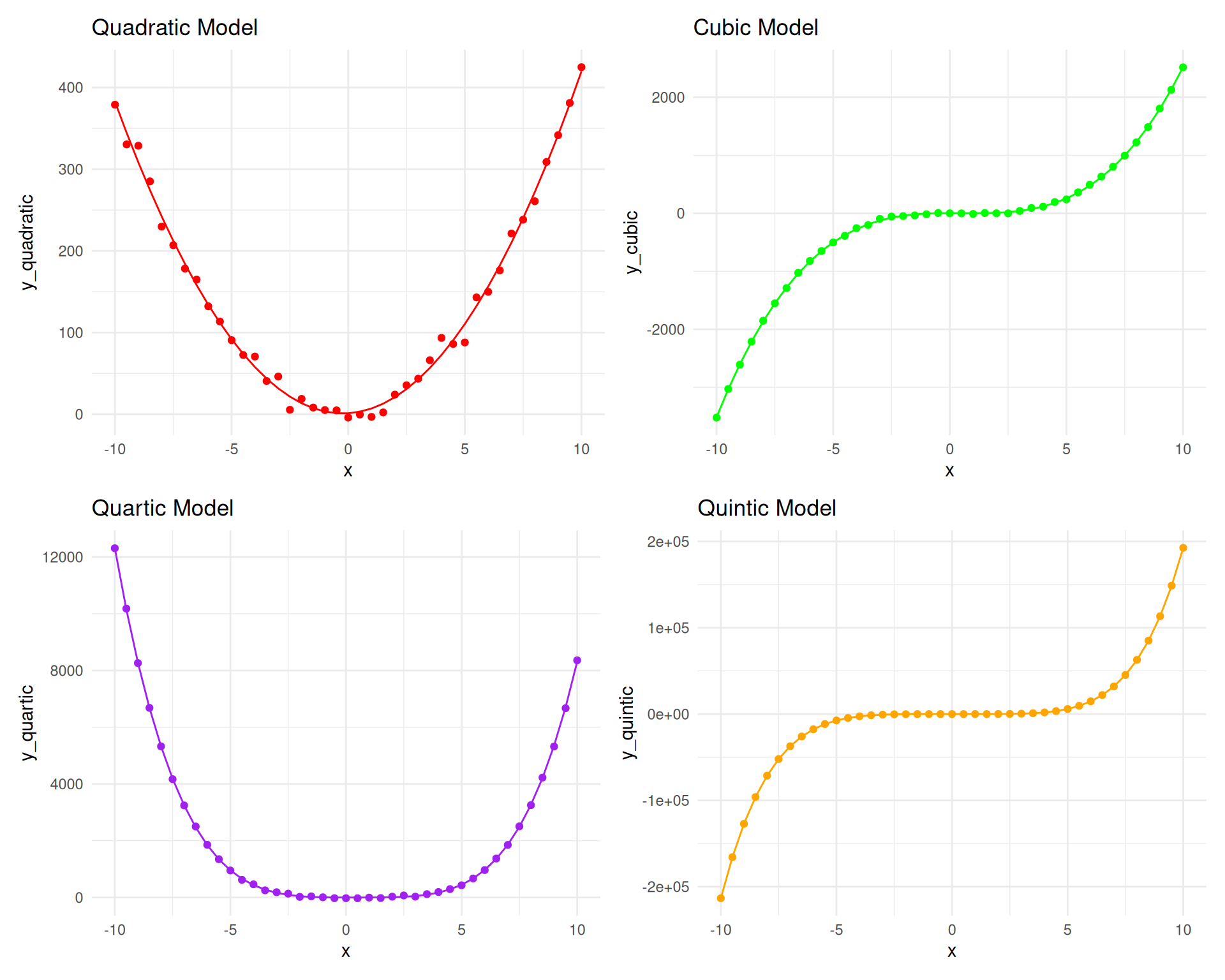
Polynomial models are versatile tools for modeling a wide range of relationships. By choosing the appropriate degree and considering the number of variables, polynomial models can capture complex patterns and provide valuable insights in various fields. When fitting polynomial models, it is essential to consider the trade-off between model complexity and overfitting. By evaluating the model’s performance and selecting the best-fitting polynomial, researchers and analysts can gain deeper insights into the underlying relationships in the data. Polynomial models are widely used in statistics, machine learning, physics, economics, and other disciplines to model nonlinear relationships and make predictions based on the data. This tutorial has provided an overview of polynomial models, their applications, and how to fit different types of polynomial models in R.
Here are some useful resources related to polynomial models and polynomial regression tutorials: