5. Multinomial Logistic Regression

Multinomial Logistic Regression is an essential statistical technique for predicting categorical outcomes where the response variable has more than two classes. It’s widely used in various fields, such as healthcare, marketing, and social sciences, to model and interpret multi-class problems such as customer preferences, diagnosis predictions, and product category classification. This tutorial will guide you through the essentials of multinomial logistic regression, from building a model from scratch in R to leveraging the {nnet} package for a more efficient approach.

Oberview

Multinomial Logistic Regression is used to model the relationship between multiple independent variables and a categorical dependent variable with more than two possible outcome categories or nominal outcome variables. It is an extension of binary logistic regression, which deals with just two categories. In multinomial logistic regression, the dependent variable can have three or more categories, and the model estimates the probability of each category given a set of predictors. The model calculates separate equations for each category relative to a reference category. These equations are typically based on the log-odds of the probability of belonging to each category. The multinomial logistic regression model assumes that the relationship between the independent variables and the dependent variable is linear in the logit (log-odds) space. The coefficients estimated by the model represent the effect of each independent variable on the log-odds of being in each category relative to the reference category.

Interpretation of the coefficients in multinomial logistic regression can be challenging because they represent the change in log-odds relative to the reference category. Therefore, converting these coefficients into odds ratios or probabilities can help in understanding the effects of the independent variables on the outcome categories.

Multinomial Logistic Regression (MLR) is an extension of binary logistic regression used when the dependent variable $y$ is categorical with more than two levels (e.g., $C$ classes, $y \in \{1, 2, \dots, C\}$.

Input and output variables are defined as:

Input Variables: $\mathbf{x} = [x_1, x_2, \dots, x_p]^T$ (a vector of $p $ -features).
Output Variable: $y \in \{1, 2, \dots, C\}$.

Model the probability of $y$ belonging to each class $c$:

\[ P(y = c \mid \mathbf{x}) \]

such that $\sum_{c=1}^C P(y = c \mid \mathbf{x}) = 1$.

In Multinomial Logistic Model, for each class $c$, define the linear predictor $\eta_c$ as:

\[ \eta_c = \mathbf{\beta}_c^T \mathbf{x} + \beta_{c, 0} \]

where:

$\mathbf{\beta}_c$ is the coefficient vector for class $c$.
$\beta_{c, 0}$ is the intercept term for class $c$.

The probabilities are modeled using the softmax function:

\[ P(y = c \mid \mathbf{x}) = \frac{\exp(\eta_c)}{\sum_{j=1}^C \exp(\eta_j)} \]

Given a dataset of $N$ observations $\{(\mathbf{x}_i, y_i)\}_{i=1}^N$, the likelihood is: \[ \mathcal{L}(\beta) = \prod_{i=1}^N \prod_{c=1}^C \big[P(y_i = c \mid \mathbf{x}_i)\big]^{\mathbb{1}(y_i = c)} \]

Taking the log, we get the log-likelihood:

\[ \ell(\beta) = \sum_{i=1}^N \sum_{c=1}^C \mathbb{1}(y_i = c) \log\big(P(y = c \mid \mathbf{x}_i)\big) \]

Parameters $\{\mathbf{\beta}_c, \beta_{c,0}\}_{c=1}^{C-1}$ are estimated by maximizing the log-likelihood using optimization techniques like gradient descent or Newton-Raphson.

To avoid overparameterization, one class (e.g., the last class) is typically set as the reference class, and its coefficients are set to zero ($\beta_C = 0$).

Multinomial Logistic Regression from Scratch

To create a multinomial logistic regression from scratch in R, we’ll build a model that handles a response variable with three levels (e.g., categories A, B, and C), using four continuous predictors and one categorical predictor with two levels (Male and Female). Here’s a step-by-step approach:

Simulate data

Code

set.seed(123)  # For reproducibility

# Create synthetic dataset
n <- 300  # Number of observations
data <- data.frame(
  response = factor(sample(c("1", "2", "3"), n, replace = TRUE)),
  continuous1 = rnorm(n),
  continuous2 = rnorm(n),
  continuous3 = rnorm(n),
  continuous4 = rnorm(n),
  gender = factor(sample(c("Male", "Female"), n, replace = TRUE))
)

# Convert response to a factor and set reference level
data$response <- relevel(data$response, ref = "1")
head(data)

  response continuous1 continuous2 continuous3 continuous4 gender
1        3   1.9009001  -0.2043353 -0.00497512  0.81293718   Male
2        3   0.7089544   0.5583362 -1.38088679  0.41497661 Female
3        3   0.7361948   0.3242106 -1.25652688 -0.08585906   Male
4        2   1.3657766   0.6977370  0.32524572 -1.90820891   Male
5        3  -0.5762639  -1.0225731 -0.27700053  0.66325198   Male
6        2  -0.8047323  -0.1682708 -0.38901100  0.66168573   Male

Data Preparation

Code

# Data Preparation
# Encode categorical variables (using "Level1" as the baseline for response)
response_matrix <- model.matrix(~ response - 1, data = data)
gender_matrix <- model.matrix(~ gender - 1, data = data)

# Check dimensions of response_matrix and gender_matrix
print(dim(response_matrix))  # Expected: n x 3 (for three levels of response)

[1] 300   3

Code

print(dim(gender_matrix))    # Expected: n x 2 (for two levels of gender, one baseline)

[1] 300   2

Define Log-Likelihood Function

The log-likelihood function is a fundamental concept in statistics, particularly in maximum likelihood estimation (MLE). It measures how well a statistical model explains a set of observations, and it’s central to estimating the parameters of a model that are most likely to have produced the observed data.

Code

# Define Log-Likelihood Function
log_likelihood <- function(params, response_matrix, X) {
  # Reshape params into a matrix with dimensions for each predictor and response level
  beta <- matrix(params, ncol = 2, byrow = TRUE)
  eta <- X %*% beta
  p <- exp(eta) / (1 + rowSums(exp(eta)))
  
  # Add a baseline category (1 - rowSums(p)) for Level1 as reference
  p <- cbind(1 - rowSums(p), p)
  
  # Negative log-likelihood calculation
  ll <- -sum(response_matrix * log(p))
  return(ll)
}

Combine Predictors

Code

# Combine Predictors
X <- cbind(1, X1=data$x1, X2=data$x2, X3=data$x3, X4=data$x4, Gender=gender_matrix[, 2])

Optimization for MLE

The optim() function in R is a general-purpose optimization function often used to find the values of parameters that maximize (or minimize) a function. In the context of maximum likelihood estimation (MLE), optim() is typically used to maximize the log-likelihood function and find the parameter estimates that best explain the observed data.

Code

# Optimization for MLE
# Initialize parameters
initial_params <- rep(0, ncol(X) * 2)  # Adjust for two response levels (Level2 and Level3)
fit <- optim(initial_params, log_likelihood, response_matrix = response_matrix, X = X, method = "BFGS", hessian = TRUE)

Summary of the model

Code

# Extract coefficients and reshape
coefficients <- matrix(fit$par, ncol = 2, byrow = TRUE)
colnames(coefficients) <- c("Level2", "Level3")
rownames(coefficients) <- colnames(X)  # Ensure row names are correctly set

#Compute Standard Errors and Z-Statistics
# Invert Hessian to get variance-covariance matrix, then take the square root of diagonal for SEs
standard_errors <- sqrt(diag(solve(fit$hessian)))

# Compute z-statistics
z_stats <- coefficients / matrix(standard_errors, ncol = 2, byrow = TRUE)

summary_table <- data.frame(
  Predictor = rep(rownames(coefficients), each = ncol(coefficients)),
  Level = rep(colnames(coefficients), times = nrow(coefficients)),
  Coefficient = as.vector(coefficients),
  Std_Error = standard_errors,
  Z_Statistic = as.vector(z_stats)
  )
# Display summary table
print(summary_table)

  Predictor  Level Coefficient Std_Error Z_Statistic
1           Level2 -0.09097131 0.2134213  -0.4262522
2           Level3 -0.07333172 0.2074024  -0.2616366
3    Gender Level2  0.02150648 0.2802808   0.1036945
4    Gender Level3 -0.44996116 0.2853473  -1.5768896

Relative Risk Ratios (RRRs)

In the context of multinomial logistic regression, the concept of relative risk ratios (RRRs) can be interpreted similarly to odds ratios in binary logistic regression. RRRs quantify the relative change in the odds of being in one category compared to a reference category, for a one-unit change in the predictor variable.

To obtain the relative risk ratios, you exponentiate the coefficients:

\[ \text{RRR}{j, k} = e^{\beta{jk}} \]

Where: - $\text{RRR}{j, k}$ is the relative risk ratio for predictor $j$ and category $k$,

$\beta{jk}$ is the coefficient for predictor $j$ and category $k$ ).

These relative risk ratios quantify how much the odds of being in category $k$ change for a one-unit increase in the predictor variable $X_j$, relative to the reference category. You can interpret a relative risk ratio of 1 as indicating no change in the odds of being in category $k$ for a one-unit change in the predictor variable. A relative risk ratio greater than 1 indicates an increase in the odds, while a ratio less than 1 indicates a decrease in the odds.

We can extract the coefficients from the model object and exponentiate them to obtain the relative risk ratios. This will give you the relative risk ratios for each predictor variable and each category of the dependent variable in the multinomial logistic regression model.

Code

# Calculate Relative Risk Ratios (RRRs)
rrr <- exp(coefficients)
risk_table <- data.frame(
  Predictor = rep(rownames(coefficients), each = ncol(coefficients)),
  Level = rep(colnames(coefficients), times = nrow(coefficients)),
  RRR = as.vector(rrr)
)
print(risk_table)

  Predictor  Level       RRR
1           Level2 0.9130439
2           Level3 0.9292925
3    Gender Level2 1.0217394
4    Gender Level3 0.6376529

Prediction and Evaluation

Code

predict_probs <- function(X, coefficients) {
  linear_preds <- X %*% coefficients
  probs <- cbind(exp(linear_preds), 1)
  probs <- probs / rowSums(probs)
  return(probs)
}

probs <- predict_probs(X, coefficients)
predicted_classes <- apply(probs, 1, which.max)

Code

# Accuracy
accuracy <- mean(predicted_classes == data$response )
cat("Accuracy:", accuracy, "\n")

Accuracy: 0.2833333

Code

# Confusion matrix
confusion_matrix <- table(Predicted = predicted_classes, Actual = data$response )
print(confusion_matrix)

         Actual
Predicted  1  2  3
        2 46 42 47
        3 66 56 43

Multinomial Logistic Regression in R

Multinomial Logistic Regression in R can be implemented using the multinom() function from the {nnet} package. This function allows us to fit a logistic regression model when the outcome variable has more than two categories.

Install Required R Packages

Code

packages <- c(
  "tidyverse", 
  "plyr", 
  "rstatix", 
  "gtsummary",
  "performance",
  "sjPlot", 
  "marginaleffects",
  "ggeffects", 
  "ggstatsplot",
  "kableExtra",
  "MASS",
  "nnet"
)

#| warning: false
#| error: false

# Install missing packages
new_packages <- packages[!(packages %in% installed.packages()[,"Package"])]
if(length(new_packages)) install.packages(new_packages)

# Verify installation
cat("Installed packages:\n")
print(sapply(packages, requireNamespace, quietly = TRUE))

Load R-packages

Code

# Load packages with suppressed messages
invisible(lapply(packages, function(pkg) {
  suppressPackageStartupMessages(library(pkg, character.only = TRUE))
}))

Code

# Check loaded packages
cat("Successfully loaded packages:\n")

Successfully loaded packages:

Code

print(search()[grepl("package:", search())])

 [1] "package:nnet"            "package:MASS"           
 [3] "package:kableExtra"      "package:ggstatsplot"    
 [5] "package:ggeffects"       "package:marginaleffects"
 [7] "package:sjPlot"          "package:performance"    
 [9] "package:gtsummary"       "package:rstatix"        
[11] "package:plyr"            "package:lubridate"      
[13] "package:forcats"         "package:stringr"        
[15] "package:dplyr"           "package:purrr"          
[17] "package:readr"           "package:tidyr"          
[19] "package:tibble"          "package:ggplot2"        
[21] "package:tidyverse"       "package:stats"          
[23] "package:graphics"        "package:grDevices"      
[25] "package:utils"           "package:datasets"       
[27] "package:methods"         "package:base"

Data

In this tutorial, we will be using health_insurance data.

The health_insurance data set consists of the following fields:

product: The choice of product of the individual — A, B or C
age: The age of the individual when they made the choice
gender: The gender of the individual as stated when they made the choice
household: The number of people living with the individual in the same household at the time of the choice
position_level: Position level in the company at the time they made the choice, where 1 is is the lowest and 5 is the highest
absent: The number of days the individual was absent from work in the year prior to the choice

Full data set is available for download can download from my Dropbox or from my Github accounts.

We will use read_csv() function of {readr} package to import data as a tidy data.

Code

# Load data
mf<-read_csv("https://github.com/zia207/r-colab/raw/main/Data/Regression_analysis/health_insurance.csv") |> 
  glimpse()

Rows: 1,448
Columns: 6
$ product        <chr> "C", "A", "C", "A", "A", "A", "A", "B", "C", "B", "B", …
$ age            <dbl> 57, 21, 66, 36, 23, 31, 37, 37, 55, 66, 58, 62, 31, 45,…
$ household      <dbl> 2, 7, 7, 4, 0, 5, 3, 0, 3, 2, 1, 2, 2, 5, 3, 5, 4, 7, 7…
$ position_level <dbl> 2, 2, 2, 2, 2, 1, 3, 3, 3, 4, 2, 2, 2, 2, 4, 4, 4, 4, 4…
$ gender         <chr> "Male", "Male", "Male", "Female", "Male", "Male", "Male…
$ absent         <dbl> 10, 7, 1, 6, 11, 14, 12, 25, 3, 18, 1, 25, 0, 10, 20, 2…

Convert to Factor

Code

mf$product <- as.factor(mf$product)
mf$gender <- as.factor(mf$gender)
levels(mf$gender)

[1] "Female" "Male"

Summary Statistics

Code

mf |> 
  # select variables
  dplyr::select (age,  household,  
                position_level, 
                absent,
                gender) |>  
  rstatix::get_summary_stats (type = "common")

# A tibble: 4 × 10
  variable           n   min   max median   iqr  mean    sd    se    ci
  <fct>          <dbl> <dbl> <dbl>  <dbl> <dbl> <dbl> <dbl> <dbl> <dbl>
1 age             1448    21    67     37    23 40.9  13.5  0.356 0.698
2 household       1448     0     7      3     3  3.26  2.23 0.059 0.115
3 position_level  1448     1     5      3     2  2.90  1.22 0.032 0.063
4 absent          1448     0    31     15    13 14.5   8.11 0.213 0.418

Box/Violine Plots

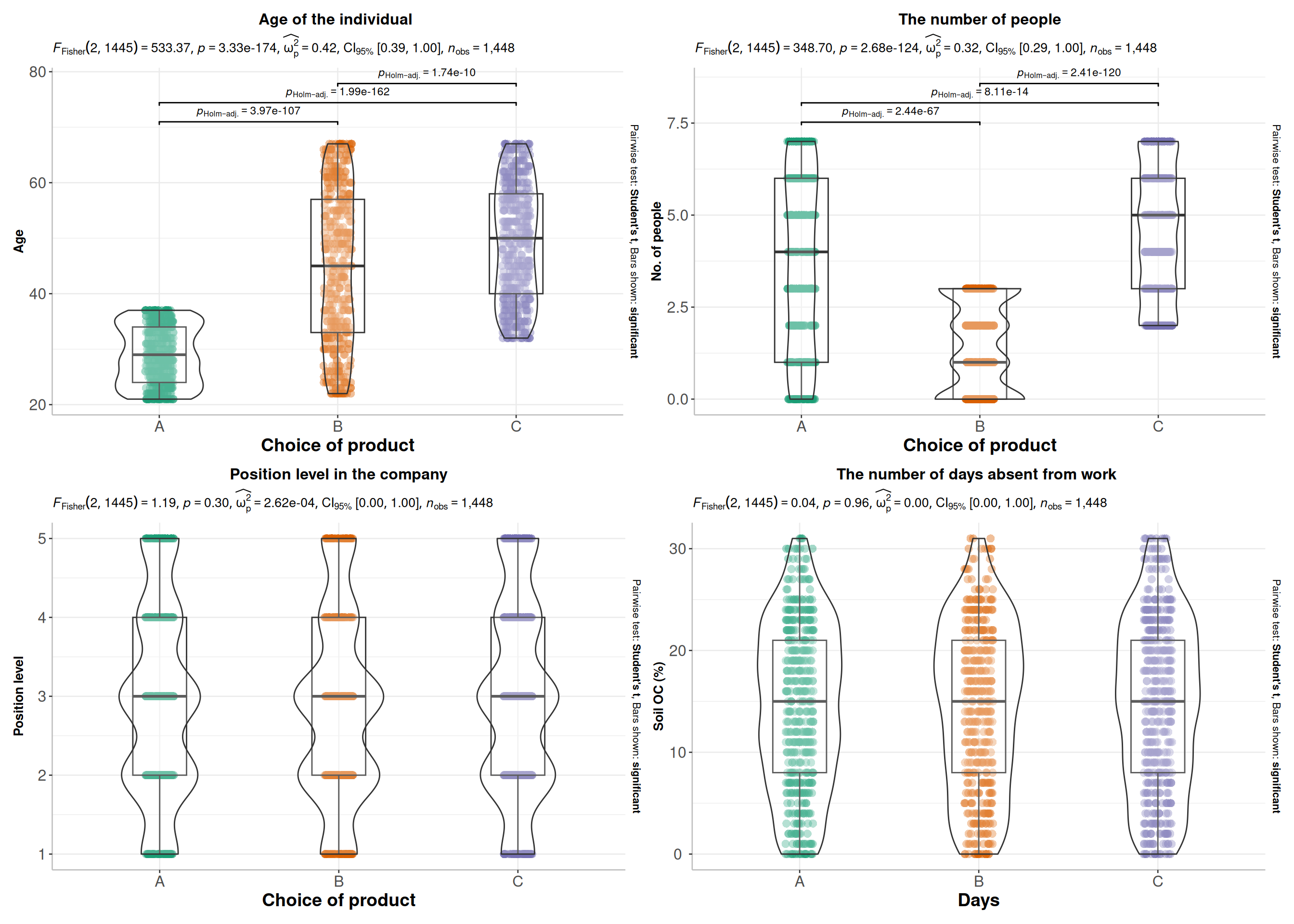
We can create a nice looking plots with results of ANOVA and post-hoc tests on the same plot (directly on the boxplots). We will use gbetweenstats() function of {ggstatsplot} package:

Code

p1<-ggstatsplot::ggbetweenstats(
  data = mf,
  x = product,
  y = age,
  ylab = "Age",
  xlab = "Choice of product",
  type = "parametric", # ANOVA or Kruskal-Wallis
  var.equal = TRUE, # ANOVA or Welch ANOVA
  plot.type = "box",
  pairwise.comparisons = TRUE,
  pairwise.display = "significant",
  centrality.plotting = FALSE,
  bf.message = FALSE
)+
# add plot title
ggtitle("Age of the individual ") +
   theme(
    # center the plot title
    plot.title = element_text(hjust = 0.5),
    axis.line = element_line(colour = "gray"),
    # axis title font size
    axis.title.x = element_text(size = 14), 
    # X and  axis font size
    axis.text.y=element_text(size=12,vjust = 0.5, hjust=0.5),
    axis.text.x = element_text(size=12))

p2<-ggstatsplot::ggbetweenstats(
  data = mf,
  x = product,
  y = household,
  ylab = "No. of people",
  xlab = "Choice of product",
  type = "parametric", # ANOVA or Kruskal-Wallis
  var.equal = TRUE, # ANOVA or Welch ANOVA
  plot.type = "box",
  pairwise.comparisons = TRUE,
  pairwise.display = "significant",
  centrality.plotting = FALSE,
  bf.message = FALSE
)+
# add plot title
ggtitle("The number of people") +
   theme(
    # center the plot title
    plot.title = element_text(hjust = 0.5),
    axis.line = element_line(colour = "gray"),
    # axis title font size
    axis.title.x = element_text(size = 14), 
    # X and  axis font size
    axis.text.y=element_text(size=12,vjust = 0.5, hjust=0.5),
    axis.text.x = element_text(size=12))

p3<-ggstatsplot::ggbetweenstats(
  data = mf,
  x = product,
  y = position_level,
  ylab = "Position level",
  xlab = "Choice of product",
  type = "parametric", # ANOVA or Kruskal-Wallis
  var.equal = TRUE, # ANOVA or Welch ANOVA
  plot.type = "box",
  pairwise.comparisons = TRUE,
  pairwise.display = "significant",
  centrality.plotting = FALSE,
  bf.message = FALSE
)+
# add plot title
ggtitle("Position level in the company") +
   theme(
    # center the plot title
    plot.title = element_text(hjust = 0.5),
    axis.line = element_line(colour = "gray"),
    # axis title font size
    axis.title.x = element_text(size = 14), 
    # X and  axis font size
    axis.text.y=element_text(size=12,vjust = 0.5, hjust=0.5),
    axis.text.x = element_text(size=12))


p4<-ggstatsplot::ggbetweenstats(
  data = mf,
  x = product,
  y = absent,
  ylab = "Soil OC (%)",
  xlab = "Days",
  type = "parametric", # ANOVA or Kruskal-Wallis
  var.equal = TRUE, # ANOVA or Welch ANOVA
  plot.type = "box",
  pairwise.comparisons = TRUE,
  pairwise.display = "significant",
  centrality.plotting = FALSE,
  bf.message = FALSE
)+
# add plot title
ggtitle("The number of days absent from work ") +
   theme(
    # center the plot title
    plot.title = element_text(hjust = 0.5),
    axis.line = element_line(colour = "gray"),
    # axis title font size
    axis.title.x = element_text(size = 14), 
    # X and  axis font size
    axis.text.y=element_text(size=12,vjust = 0.5, hjust=0.5),
    axis.text.x = element_text(size=12))

Code

(p1|p2)/(p3|p4)

Split Data

Code

seeds = 11076
tr_prop = 0.70
# training data (70% data)
train= ddply(mf,.(product, gender ),
                 function(., seed) { set.seed(seed); .[sample(1:nrow(.), trunc(nrow(.) * tr_prop)), ] }, seed = 101)
test = ddply(mf, .(product , gender),
            function(., seed) { set.seed(seed); .[-sample(1:nrow(.), trunc(nrow(.) * tr_prop)), ] }, seed = 101)
print(prop.table(table(train$product)))


        A         B         C 
0.3405941 0.3158416 0.3435644

Code

print(prop.table(table(test$product)))


        A         B         C 
0.3401826 0.3150685 0.3447489

Fit a Multinomial Model

Before we fit multinom() function from the {nnet} the model, we need to make sure our reference level is defined.

Code

train$product <- relevel(train$product, ref = "A")
test$product <- relevel(test$product, ref = "A")

Code

fit.multinom<-nnet::multinom(product~., data= train, Hessain = T)

# weights:  21 (12 variable)
initial  value 1109.598412 
iter  10 value 702.581012
iter  20 value 517.407633
final  value 517.303192 
converged

Model Summary

Code

summary(fit.multinom)

Call:
nnet::multinom(formula = product ~ ., data = train, Hessain = T)

Coefficients:
  (Intercept)       age  household position_level genderMale      absent
B   -4.959751 0.2590934 -1.0032411     -0.4503334 -2.3320817 0.009837554
C  -10.431411 0.2821310  0.1840855     -0.3119368  0.1063362 0.014618147

Std. Errors:
  (Intercept)        age household position_level genderMale     absent
B   0.6313473 0.01959831 0.0864775     0.10673739  0.2774411 0.01561814
C   0.7534633 0.01980966 0.0594349     0.09886281  0.2345722 0.01506402

Residual Deviance: 1034.606 
AIC: 1058.606

Z-statistics of Coefficients

To determine whether specific input variables are significant we will need to calculate the p-values of the coefficients manually by calculating the z-statistics.

Code

z_stats <- summary(fit.multinom)$coefficients/
  summary(fit.multinom)$standard.errors
# convert to p-values
p_values <- (1 - pnorm(abs(z_stats)))*2

# display p-values in transposed data frame
data.frame(t(p_values))

                          B           C
(Intercept)    3.996803e-15 0.000000000
age            0.000000e+00 0.000000000
household      0.000000e+00 0.001953166
position_level 2.453035e-05 0.001603610
genderMale     0.000000e+00 0.650318459
absent         5.287731e-01 0.331846545

If we want to display our classic summary results with each predictor variable as a row and include confidence intervals, we can use the tidy() function. In the results table, the first column represents the dependent variable outcome, and the second column represents the predictor variable, which corresponds to the coefficient in the estimate column.

Code

tidy(fit.multinom, conf.int = TRUE)

# A tibble: 12 × 8
   y.level term         estimate std.error statistic  p.value conf.low conf.high
   <chr>   <chr>           <dbl>     <dbl>     <dbl>    <dbl>    <dbl>     <dbl>
 1 B       (Intercept)  -4.96e+0    0.631     -7.86  3.97e-15  -6.20     -3.72  
 2 B       age           2.59e-1    0.0196    13.2   6.71e-40   0.221     0.298 
 3 B       household    -1.00e+0    0.0865   -11.6   4.06e-31  -1.17     -0.834 
 4 B       position_le… -4.50e-1    0.107     -4.22  2.45e- 5  -0.660    -0.241 
 5 B       genderMale   -2.33e+0    0.277     -8.41  4.25e-17  -2.88     -1.79  
 6 B       absent        9.84e-3    0.0156     0.630 5.29e- 1  -0.0208    0.0404
 7 C       (Intercept)  -1.04e+1    0.753    -13.8   1.37e-43 -11.9      -8.95  
 8 C       age           2.82e-1    0.0198    14.2   5.02e-46   0.243     0.321 
 9 C       household     1.84e-1    0.0594     3.10  1.95e- 3   0.0676    0.301 
10 C       position_le… -3.12e-1    0.0989    -3.16  1.60e- 3  -0.506    -0.118 
11 C       genderMale    1.06e-1    0.235      0.453 6.50e- 1  -0.353     0.566 
12 C       absent        1.46e-2    0.0151     0.970 3.32e- 1  -0.0149    0.0441

And if you dislike the inability to view the entire “term” column, you can utilize kable() and kable_styling() to present it as an html table.

Code

tidy(fit.multinom, conf.int = TRUE) %>% 
  kable() %>% 
  kable_styling("basic", full_width = FALSE)

y.level	term	estimate	std.error	statistic	p.value	conf.low	conf.high
B	(Intercept)	-4.9597508	0.6313473	-7.8558200	0.0000000	-6.1971688	-3.7223328
B	age	0.2590934	0.0195983	13.2201880	0.0000000	0.2206814	0.2975053
B	household	-1.0032411	0.0864775	-11.6011813	0.0000000	-1.1727339	-0.8337484
B	position_level	-0.4503334	0.1067374	-4.2190779	0.0000245	-0.6595348	-0.2411319
B	genderMale	-2.3320817	0.2774411	-8.4056830	0.0000000	-2.8758562	-1.7883072
B	absent	0.0098376	0.0156181	0.6298800	0.5287731	-0.0207734	0.0404485
C	(Intercept)	-10.4314112	0.7534633	-13.8446179	0.0000000	-11.9081721	-8.9546503
C	age	0.2821310	0.0198097	14.2420911	0.0000000	0.2433048	0.3209573
C	household	0.1840855	0.0594349	3.0972629	0.0019532	0.0675952	0.3005758
C	position_level	-0.3119368	0.0988628	-3.1552494	0.0016036	-0.5057044	-0.1181693
C	genderMale	0.1063362	0.2345722	0.4533198	0.6503185	-0.3534168	0.5660892
C	absent	0.0146181	0.0150640	0.9704012	0.3318465	-0.0149068	0.0441431

Relative Risk Ratios (RRRs)

Code

# Extract coefficients
coefficients <- coef(fit.multinom)
# Exponentiate coefficients to obtain relative risk ratios
RRRs <- exp(coefficients)
# Print relative risk ratios
print(RRRs)

   (Intercept)      age household position_level genderMale   absent
B 7.014676e-03 1.295755  0.366689      0.6374156 0.09709342 1.009886
C 2.949142e-05 1.325952  1.202119      0.7320278 1.11219574 1.014726

The tbl_regression() function from the {gtsummary} package takes a regression model object as input and produces a formatted table with Odd-ratio and confidence interval.

Code

tbl_regression(fit.multinom,  exp = TRUE)

Characteristic	OR	95% CI	p-value
B
age	1.30	1.25, 1.35	<0.001
household	0.37	0.31, 0.43	<0.001
position_level	0.64	0.52, 0.79	<0.001
gender
Female	—	—
Male	0.10	0.06, 0.17	<0.001
absent	1.01	0.98, 1.04	0.5
C
age	1.33	1.28, 1.38	<0.001
household	1.20	1.07, 1.35	0.002
position_level	0.73	0.60, 0.89	0.002
gender
Female	—	—
Male	1.11	0.70, 1.76	0.7
absent	1.01	0.99, 1.05	0.3
Abbreviations: CI = Confidence Interval, OR = Odds Ratio

The tab_model() function of {sjPlot} package also creates HTML tables from regression models:

Code

tab_model(fit.multinom)

	product
Predictors	Odds Ratios	CI	p	Response
(Intercept)	0.01	0.00 – 0.02	<0.001	B
age	1.30	1.25 – 1.35	<0.001	B
household	0.37	0.31 – 0.43	<0.001	B
position level	0.64	0.52 – 0.79	<0.001	B
gender [Male]	0.10	0.06 – 0.17	<0.001	B
absent	1.01	0.98 – 1.04	0.529	B
(Intercept)	0.00	0.00 – 0.00	<0.001	C
age	1.33	1.28 – 1.38	<0.001	C
household	1.20	1.07 – 1.35	0.002	C
position level	0.73	0.60 – 0.89	0.002	C
gender [Male]	1.11	0.70 – 1.76	0.650	C
absent	1.01	0.99 – 1.05	0.332	C
Observations	1010
R² / R² adjusted	0.533 / 0.533

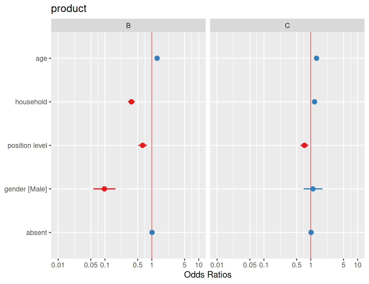
plot_model() function of {sjPlot} package creates plots the estimates from logistic model:

Code

plot_model(fit.multinom, vline.color = "red")

Model Performance

Code

performance::performance(fit.multinom)

Can't calculate log-loss.

# Indices of model performance

AIC      |     AICc |      BIC |    R2 | R2 (adj.) |  RMSE | Sigma
------------------------------------------------------------------
1058.606 | 1058.919 | 1117.619 | 0.533 |     0.533 | 0.324 | 1.018

Overall Training Accuracy

Code

# Calculate the predicted classes for the training set
train$Pred.Class <- predict(fit.multinom, train)
# Calculate training accuracy
train.accuracy <- mean(train$Pred.Class == train$product)
cat("Training Accuracy: ", train.accuracy, "\n")

Training Accuracy:  0.7782178

Confusion Matrix

Code

# Create a confusion matrix
conf.matrix.train <- table(Predicted = train$Pred.Class, Actual = train$product)
conf.matrix.train

         Actual
Predicted   A   B   C
        A 284  46  47
        B  39 246  44
        C  21  27 256

In-class Accuracy or Per-class Accuracy

Code

# Calculate in-class accuracy
in_class_accuracy.train <- diag(conf.matrix.train) / colSums(conf.matrix.train)

# Display in-class accuracy for each class
cat("In-Class Accuracy for each class:\n")

In-Class Accuracy for each class:

Code

print(round(in_class_accuracy.train* 100, 2))

    A     B     C 
82.56 77.12 73.78

Marginal Effects and Adjusted Predictions

The presentation of regression models, usually shown in tables, is a clear and easy way to interpret results. However, for more complex models that include interaction or transformed terms, such as quadratic or spline terms, using raw regression coefficients may be less effective. This can make it challenging to understand outcomes. In these cases, adjusted predictions or marginal means are a better solution. Using visual aids can also help to understand these effects or predictions, providing an intuitive understanding of the relationship between predictors and outcomes, even for complex models.

we get the same marginal effect using avg_slopes() function from the {marginaleffects} package

Code

marginaleffects::avg_slopes(fit.multinom, variables = "age")


 Group Estimate Std. Error     z Pr(>|z|)     S    2.5 %  97.5 %
     A -0.02611   0.000728 -35.9   <0.001 933.1 -0.02753 -0.0247
     B  0.00962   0.000636  15.1   <0.001 169.3  0.00837  0.0109
     C  0.01649   0.000601  27.4   <0.001 548.4  0.01531  0.0177

Term: age
Type:  probs 
Comparison: dY/dX

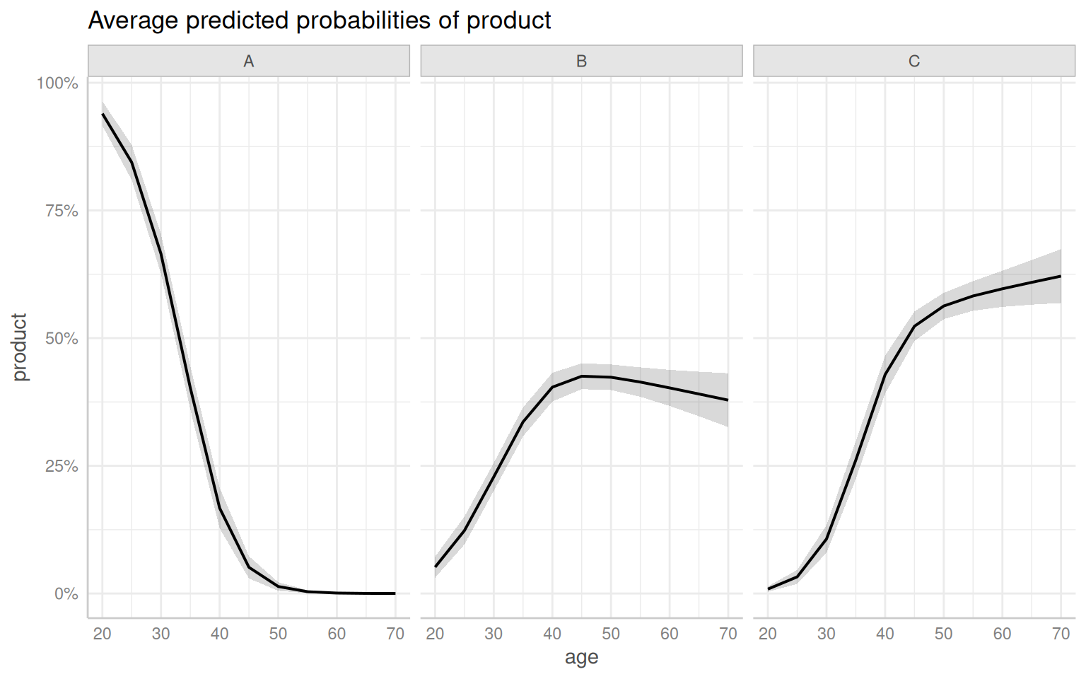
To calculate marginal effects and adjusted predictions, the predict_response() function of {ggeffects} package is used. This function can return three types of predictions, namely, conditional effects, marginal effects or marginal means, and average marginal effects or counterfactual predictions. You can set the type of prediction you want by using the margin argument.

Code

effect<-ggeffects::predict_response(fit.multinom, "age", margin = "empirical")
plot(effect)

Code

effect$predicted[2] - effect$predicted[1]

[1] -0.8878722

Code

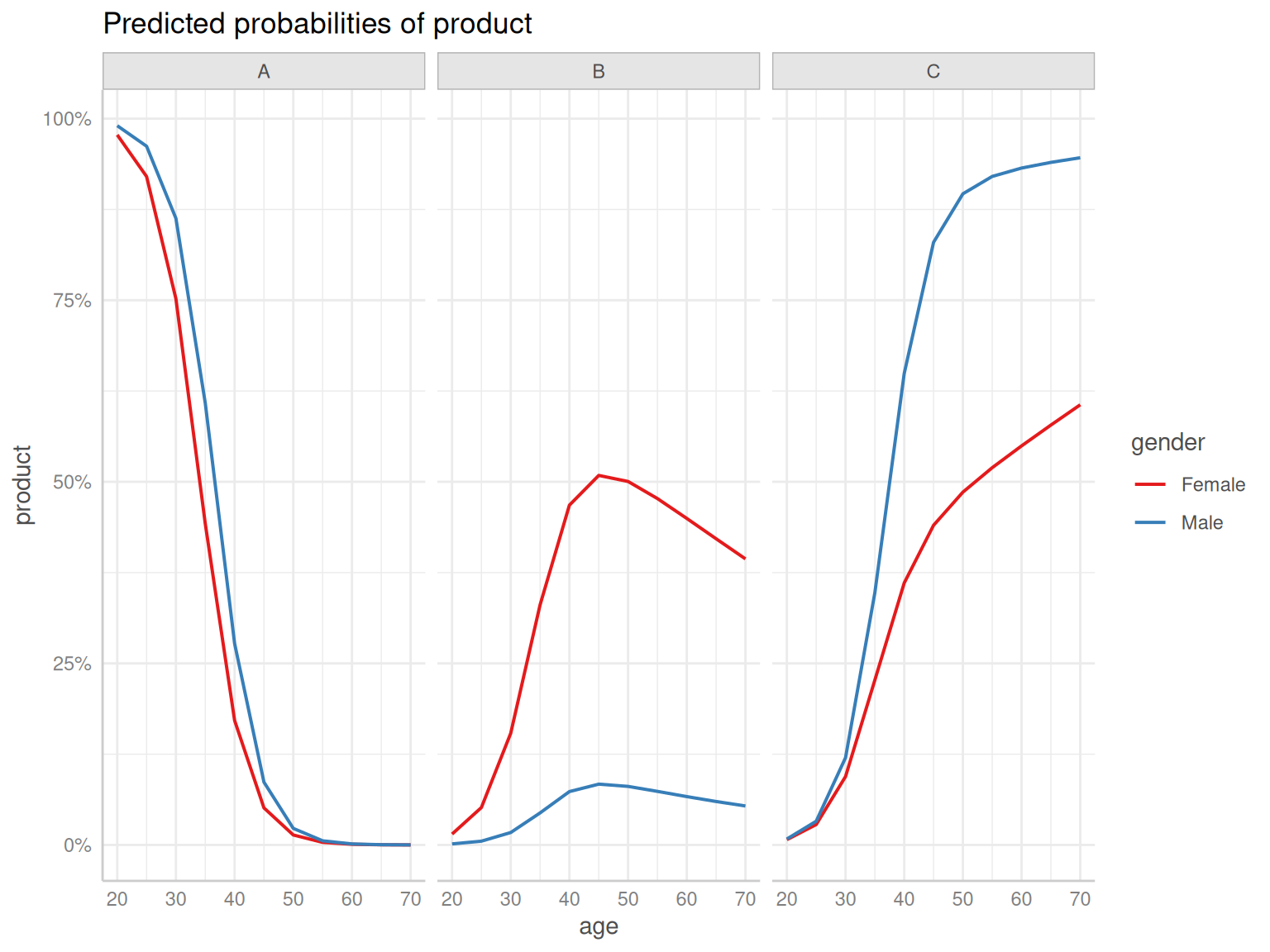
age.gender <- predict_response(fit.multinom, terms = c("age", "gender"))
plot(age.gender, facets = TRUE)

Cross-Validation

Code

# Set a seed for reproducibility
set.seed(123)
mf$product <- relevel(mf$product, ref = "A")

# Define the number of folds for cross-validation
k <- 10
folds <- sample(rep(1:k, length.out = nrow(mf)))

# Initialize a vector to store accuracy
accuracy <- numeric(k)

# Perform k-fold cross-validation
for(i in 1:k) {
  # Split the data into training and test sets
  train_data <- mf[folds != i, ]
  test_data <- mf[folds == i, ]
  
  # Fit the multinomial logistic regression model
  model <- multinom(product ~ ., data = train_data)
  
  # Make predictions on the test set
  predictions <- predict(model, newdata = test_data)
  
  # Calculate accuracy
  accuracy[i] <- mean(predictions == test_data$product)
}

# weights:  21 (12 variable)
initial  value 1431.491812 
iter  10 value 845.553727
iter  20 value 667.198403
final  value 667.143901 
converged
# weights:  21 (12 variable)
initial  value 1431.491812 
iter  10 value 847.246088
iter  20 value 668.901238
final  value 668.810030 
converged
# weights:  21 (12 variable)
initial  value 1431.491812 
iter  10 value 853.565387
iter  20 value 668.226170
final  value 668.169797 
converged
# weights:  21 (12 variable)
initial  value 1431.491812 
iter  10 value 867.663926
iter  20 value 658.594898
final  value 658.533703 
converged
# weights:  21 (12 variable)
initial  value 1431.491812 
iter  10 value 857.381406
iter  20 value 674.130530
final  value 674.076607 
converged
# weights:  21 (12 variable)
initial  value 1431.491812 
iter  10 value 828.673560
iter  20 value 653.453615
final  value 653.401842 
converged
# weights:  21 (12 variable)
initial  value 1431.491812 
iter  10 value 841.848425
iter  20 value 667.021539
final  value 666.943761 
converged
# weights:  21 (12 variable)
initial  value 1431.491812 
iter  10 value 854.993861
iter  20 value 672.018579
final  value 671.962795 
converged
# weights:  21 (12 variable)
initial  value 1432.590424 
iter  10 value 850.880994
iter  20 value 665.401801
final  value 665.327819 
converged
# weights:  21 (12 variable)
initial  value 1432.590424 
iter  10 value 863.294019
iter  20 value 673.363592
final  value 673.293777 
converged

Code

# Calculate and print the average accuracy across all folds
average_accuracy <- mean(accuracy)
cat("Average Accuracy from Cross-Validation: ", average_accuracy, "\n")

Average Accuracy from Cross-Validation:  0.7631082

Prediction at Test Data

The predict() function for logistic models returns the default predictions of log-odds, which are probabilities on the logit scale. When type = response, the function provides the predicted probabilities.

Code

test$Pred.Class<-predict(fit.multinom, test, type = "class")

Overall Auccuracy

Code

# Calculate accuracy
test.accuracy <- mean(test$Pred.Class == test$product)
cat("Test Accuracy: ", test.accuracy , "\n")

Test Accuracy:  0.7579909

Confusion Matrix

Code

# Create a confusion matrix
conf.matrix.test <- table(Predicted = test$Pred.Class, Actual = test$product)
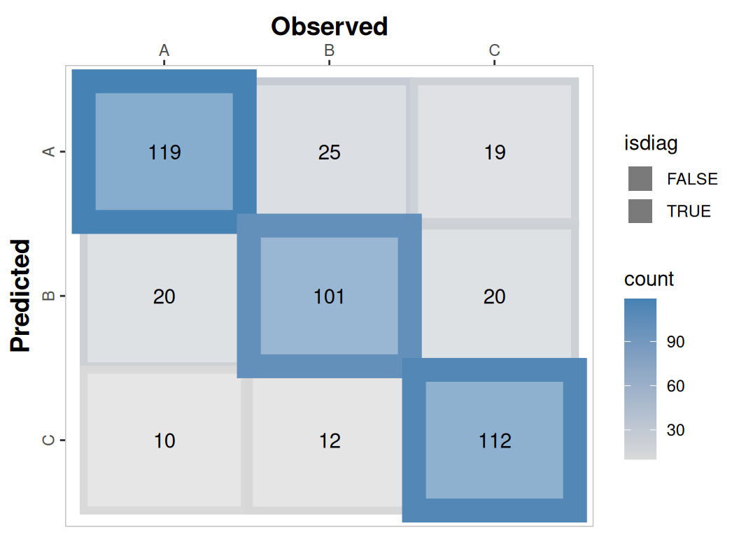
conf.matrix.test

         Actual
Predicted   A   B   C
        A 119  25  19
        B  20 101  20
        C  10  12 112

To creates a confusion matrix table or plot displaying the agreement between the observed and the predicted classes by the model use metrica:: confusion_matrix() function

Code

 test |> 
 dplyr::select(product, Pred.Class) |> 
 metrica:: confusion_matrix(obs = product, pred = Pred.Class, 
                                      plot = TRUE, 
                                      colors = c(low="grey85" , high="steelblue"), 
                                      unit = "count")

Prediction Performance Summary

Code

# Get a selected list at once with metrics_summary()
selected_class_metrics <- c("accuracy", "precision", "recall", "fscore")
test %>% 
  dplyr::select(product, Pred.Class) |> 
  metrica::metrics_summary( 
                  obs = product, pred = Pred.Class,  
                  type = "classification",
                  metrics_list = selected_class_metrics)

Warning in metrica::fscore(data = ~test %>% dplyr::select(product, Pred.Class),
: For multiclass cases, the fscore should be estimated at a class level.
Please, consider using `atom = TRUE`

Warning in metrica::agf(data = ~test %>% dplyr::select(product, Pred.Class), :
For multiclass cases, the agf should be estimated at a class level. Please,
consider using `atom = TRUE`

Warning in metrica::fmi(data = ~test %>% dplyr::select(product, Pred.Class), :
The Fowlkes-Mallows Index is not available for multiclass cases. The result has
been recorded as NaN.

Warning in metrica::preval(data = ~test %>% dplyr::select(product, Pred.Class),
: For multiclass cases, prevalence should be estimated at a class level. A NaN
has been recorded as the result. Please, use `atom = TRUE`

Warning in metrica::preval_t(data = ~test %>% dplyr::select(product, Pred.Class), : For multiclass cases, prevalence threshold should be estimated at a class level. 
      A NaN has been recorded as the result. Please, use `atom = TRUE`.

Warning in metrica::p4(data = ~test %>% dplyr::select(product, Pred.Class), :
Sorry, the p4 metric has not been generalized for multinomial cases. A NaN has
been recorded as the result

     Metric     Score
1  accuracy 0.7579909
2 precision 0.7607314
3    recall 0.7574212
4    fscore 0.7590727

In-class Accuracy or Per-class Accuracy

Code

# Calculate in-class accuracy
in_class_accuracy.test <- diag(conf.matrix.test) / colSums(conf.matrix.test)

# Display in-class accuracy for each class
cat("In-Class Accuracy for each class:\n")

In-Class Accuracy for each class:

Code

print(round(in_class_accuracy.test * 100, 2))

    A     B     C 
79.87 73.19 74.17

Summary and Conclusion

This tutorial explains how to apply multinomial logistic regression to perform multi-class classification with the nnet package. It covers data preparation, model fitting, evaluation, and interpretation of results. It also provides insights into interpreting the coefficients of the logistic regression model and discusses potential challenges. By following this tutorial, readers can gain a solid understanding of logistic regression analysis in R.

References

Session Info

Code

sessionInfo()

R version 4.4.2 (2024-10-31)
Platform: x86_64-pc-linux-gnu
Running under: Ubuntu 24.04.1 LTS

Matrix products: default
BLAS:   /usr/lib/x86_64-linux-gnu/blas/libblas.so.3.12.0 
LAPACK: /usr/lib/x86_64-linux-gnu/lapack/liblapack.so.3.12.0

locale:
 [1] LC_CTYPE=en_US.UTF-8       LC_NUMERIC=C              
 [3] LC_TIME=en_US.UTF-8        LC_COLLATE=en_US.UTF-8    
 [5] LC_MONETARY=en_US.UTF-8    LC_MESSAGES=en_US.UTF-8   
 [7] LC_PAPER=en_US.UTF-8       LC_NAME=C                 
 [9] LC_ADDRESS=C               LC_TELEPHONE=C            
[11] LC_MEASUREMENT=en_US.UTF-8 LC_IDENTIFICATION=C       

time zone: America/New_York
tzcode source: system (glibc)

attached base packages:
[1] stats     graphics  grDevices utils     datasets  methods   base     

other attached packages:
 [1] nnet_7.3-20            MASS_7.3-64            kableExtra_1.4.0      
 [4] ggstatsplot_0.13.0     ggeffects_2.2.0        marginaleffects_0.25.0
 [7] sjPlot_2.8.17          performance_0.13.0     gtsummary_2.1.0       
[10] rstatix_0.7.2          plyr_1.8.9             lubridate_1.9.4       
[13] forcats_1.0.0          stringr_1.5.1          dplyr_1.1.4           
[16] purrr_1.0.4            readr_2.1.5            tidyr_1.3.1           
[19] tibble_3.2.1           ggplot2_3.5.1          tidyverse_2.0.0       

loaded via a namespace (and not attached):
  [1] RColorBrewer_1.1-3     rstudioapi_0.17.1      jsonlite_1.9.0        
  [4] datawizard_1.0.2       correlation_0.8.7      magrittr_2.0.3        
  [7] TH.data_1.1-3          estimability_1.5.1     farver_2.1.2          
 [10] rmarkdown_2.29         minerva_1.5.10         vctrs_0.6.5           
 [13] memoise_2.0.1          paletteer_1.6.0        base64enc_0.1-3       
 [16] effectsize_1.0.0       htmltools_0.5.8.1      energy_1.7-12         
 [19] curl_6.2.1             haven_2.5.4            broom_1.0.7           
 [22] Formula_1.2-5          sjmisc_2.8.10          sass_0.4.9            
 [25] htmlwidgets_1.6.4      sandwich_3.1-1         emmeans_1.11.0        
 [28] zoo_1.8-13             cachem_1.1.0           gt_0.11.1             
 [31] commonmark_1.9.2       lifecycle_1.0.4        pkgconfig_2.0.3       
 [34] sjlabelled_1.2.0       Matrix_1.7-1           R6_2.6.1              
 [37] fastmap_1.2.0          digest_0.6.37          colorspace_2.1-1      
 [40] rematch2_2.1.2         patchwork_1.3.0        prismatic_1.1.2       
 [43] RSQLite_2.3.9          labeling_0.4.3         timechange_0.3.0      
 [46] abind_1.4-8            compiler_4.4.2         bit64_4.6.0-1         
 [49] withr_3.0.2            gsl_2.1-8              backports_1.5.0       
 [52] carData_3.0-5          metrica_2.1.0          DBI_1.2.3             
 [55] ggsignif_0.6.4         sjstats_0.19.0         tools_4.4.2           
 [58] statsExpressions_1.6.2 glue_1.8.0             grid_4.4.2            
 [61] checkmate_2.3.2        generics_0.1.3         gtable_0.3.6          
 [64] labelled_2.14.0        tzdb_0.4.0             data.table_1.17.0     
 [67] hms_1.1.3              xml2_1.3.6             car_3.1-3             
 [70] utf8_1.2.4             pillar_1.10.1          markdown_1.13         
 [73] vroom_1.6.5            splines_4.4.2          lattice_0.22-5        
 [76] survival_3.8-3         bit_4.5.0.1            tidyselect_1.2.1      
 [79] knitr_1.49             svglite_2.1.3          xfun_0.51             
 [82] stringi_1.8.4          yaml_2.3.10            boot_1.3-31           
 [85] evaluate_1.0.3         codetools_0.2-20       cli_3.6.4             
 [88] RcppParallel_5.1.10    xtable_1.8-4           parameters_0.24.2     
 [91] systemfonts_1.2.1      munsell_0.5.1          Rcpp_1.0.14           
 [94] zeallot_0.1.0          coda_0.19-4.1          parallel_4.4.2        
 [97] rstantools_2.4.0       blob_1.2.4             bayestestR_0.15.2     
[100] viridisLite_0.4.2      broom.helpers_1.20.0   mvtnorm_1.3-3         
[103] scales_1.3.0           insight_1.1.0          crayon_1.5.3          
[106] rlang_1.1.5            multcomp_1.4-28        cards_0.5.0.9000