3. Panel Regression Models fit via {panelr} Package
The panelr package in R is designed for handling and analyzing panel data, also known as longitudinal data or time-series cross-sectional data. Panel data involves repeated measurements of the same units (such as individuals, firms, or countries) over multiple time periods. The panelr package provides a user-friendly interface and functions that simplify the process of preparing, modeling, and interpreting panel data.
Overview
Panel data analysis is a common approach in social sciences, economics, and other fields where researchers are interested in studying the dynamics of individual units over time. Panel data sets are characterized by having both cross-sectional and time-series dimensions, allowing researchers to examine how variables change within and between units over time. Panel regression models are used to analyze panel data and estimate the relationships between variables while accounting for individual-specific effects and time-varying predictors. The panelr package provides a set of functions for working with panel data, including data preparation, model estimation, and interpretation.
Key Features of {panelr}
Data Preparation:
Functions to reshape data between wide and long formats, which is crucial for panel data analysis.
Handling missing data and creating lagged variables.
Modeling:
Support for various types of panel models, including fixed effects, random effects, and mixed effects models.
Easy-to-use syntax for specifying models.
Interpretation:
Functions to extract and interpret model results, including fixed effects, random effects, and overall model fit.
Visualization tools for plotting model predictions and effects.
Example Functions
The panelr package provides several functions for working with panel data, including:
Regression models
Regression models for panel data can be fit using the following functions in the panelr package:
wbm(): Panel regression models fit via multilevel modeling
wbgee(): Panel regression models fit with GEE
fdm(): Estimate first differences models using GLS
asym(): Estimate asymmetric effects models using first differences
asym_gee(): Asymmetric effects models fit with GEE
wbm_stan(): Bayesian estimation of within-between models
Panel data wrangling
Data preparation and manipulation functions in panelr include:
panel_data()as_pdata.frame()as_panel_data()as_panel() Create panel data frames
widen_panel()Convert long panel data to wide format
long_panel() Convert wide panels to long format
summary(<panel_data>) Summarize panel data frames
complete_data() Filter out entities with too few observations
model_frame() Make model frames for panel_data objects
unpanel() Convert panel_data to regular data frame
is_panel() Check if object is panel_data
Install Required R Packages
Following R packages are required to run this notebook. If any of these packages are not installed, you can install them using the code below:
Panel regression models fit via multilevel modeling
The wbm() function in the panelr package fits panel regression models using multilevel modeling. This function is useful for estimating fixed effects, random effects, and mixed effects models for panel data. The wbm() function takes a formula as input, where the dependent variable is on the left-hand side, and the independent variables are on the right-hand side. The formula can include fixed effects, random effects, and other model specifications.
Data
We use data from the WageData dataset in the palenr package to demonstrate the wbm() function. The WageData dataset come from the years 1976-1982 in the Panel Study of Income Dynamics (PSID), with information about the demographics and earnings of 595 individuals.
Code
# Load the WageData dataset from the panelr packagedata("WageData", package ="panelr")head(WageData)
panel_data() function is used to create a panel data object from the WageData dataset. The panel_data() function requires specifying the id variable (entity identifier) and the wave variable (time identifier) in the dataset. In this case, the id variable is id and the wave variable is t.
Code
wages <-panel_data(WageData, id = id, wave = t)
Fit “within-between” Model
The code below fits a weighted balanced panel model using the wbm() function from the {panelr} package. The model aims to explain the log of wages (lwage) based on several independent variables and their interactions:
The lagged value of union membership (lag(union)).
The number of weeks worked (wks).
Main effects for being Black (blk) and being female (fem).
An interaction term between being Black and lagged union membership (blk * lag(union)).
family =gaussian use this to specify GLM link families. Default is gaussian, the linear model. Other options include binomial, poisson, and negative binomial. By default argument model= "w-b", which specifies the within-between model.
MODEL INFO:
Entities: 595
Time periods: 2-7
Dependent variable: lwage
Model type: Linear mixed effects
Specification: within-between

MODEL FIT:
AIC = 1386.31, BIC = 1448.11
Pseudo-R² (fixed effects) = 0.13
Pseudo-R² (total) = 0.74
Entity ICC = 0.7

WITHIN EFFECTS:
---------------------------------------------------------
                    Est.   S.E.   t val.      d.f.      p
---------------- ------- ------ -------- --------- ------
lag(union)          0.06   0.03     2.28   2972.01   0.02
wks                -0.00   0.00    -1.51   2994.31   0.13
---------------------------------------------------------

BETWEEN EFFECTS:
---------------------------------------------------------------
                           Est.   S.E.   t val.     d.f.      p
----------------------- ------- ------ -------- -------- ------
(Intercept)                6.60   0.23    28.53   589.99   0.00
imean(lag(union))         -0.03   0.03    -0.80   589.98   0.42
imean(wks)                 0.00   0.00     0.91   589.99   0.36
blk                       -0.23   0.06    -3.85   589.98   0.00
fem                       -0.44   0.05    -8.89   589.98   0.00
---------------------------------------------------------------

CROSS-LEVEL INTERACTIONS:
-------------------------------------------------------------
                        Est.   S.E.   t val.      d.f.      p
-------------------- ------- ------ -------- --------- ------
lag(union):blk         -0.13   0.12    -1.03   2971.99   0.31
-------------------------------------------------------------

p values calculated using Satterthwaite d.f.

RANDOM EFFECTS:
------------------------------------
  Group      Parameter    Std. Dev.
---------- ------------- -----------
    id      (Intercept)     0.354
 Residual                  0.2326
------------------------------------
The output of the summary() function provides the coefficients, standard errors, t-values, and p-values for the model parameters. The wbm() function fits a within-between model with fixed effects for blk and fem, as well as an cross-level interaction term between blk and the lagged value of union. imean() is an internal function that calculates the individual-level mean, which represents the between-subjects effects of the time-varying predictors. The wbm() function also provides the overall model fit statistics, including the marginal and conditional R-squared values.
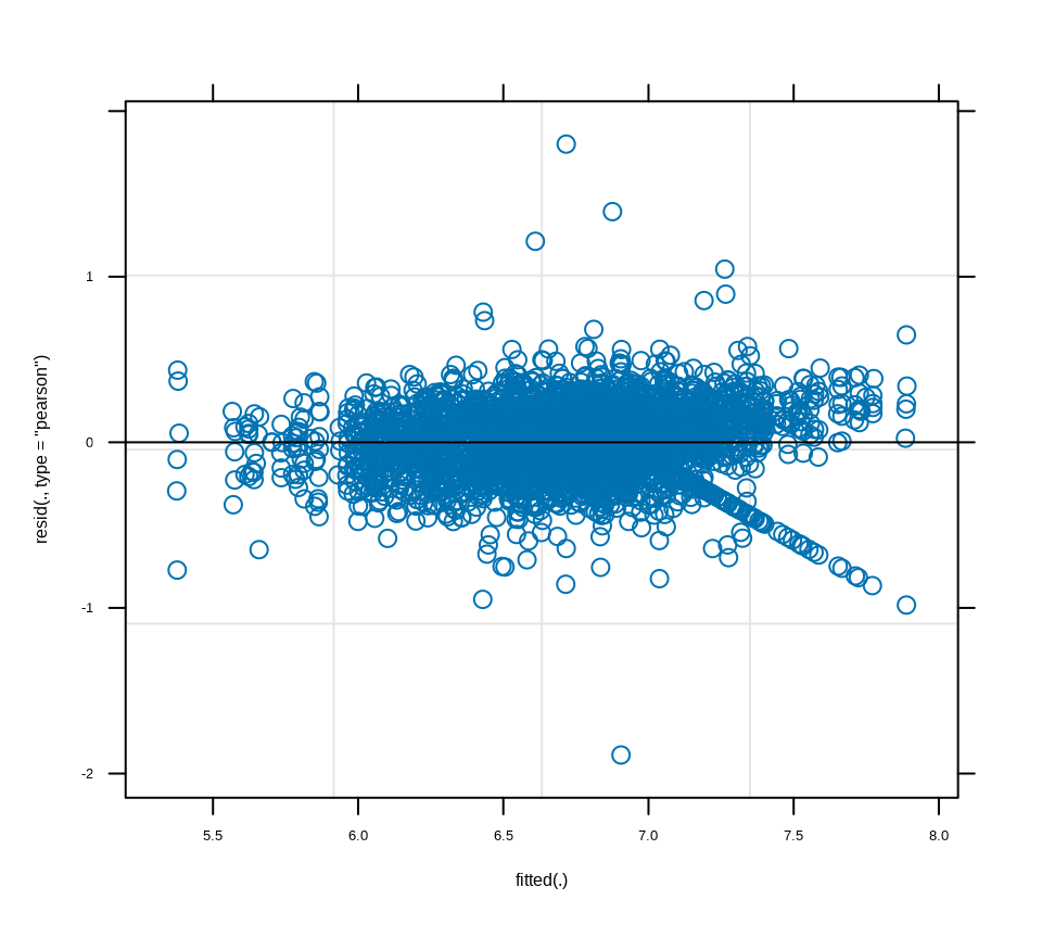
Model Diagnostics
The wbm() function also provides diagnostic plots to assess the model assumptions and identify potential issues. The plot() function can be used to visualize the model diagnostics, including the residuals, fitted values, and QQ plot of the residuals.
Code
plot(model.wb)
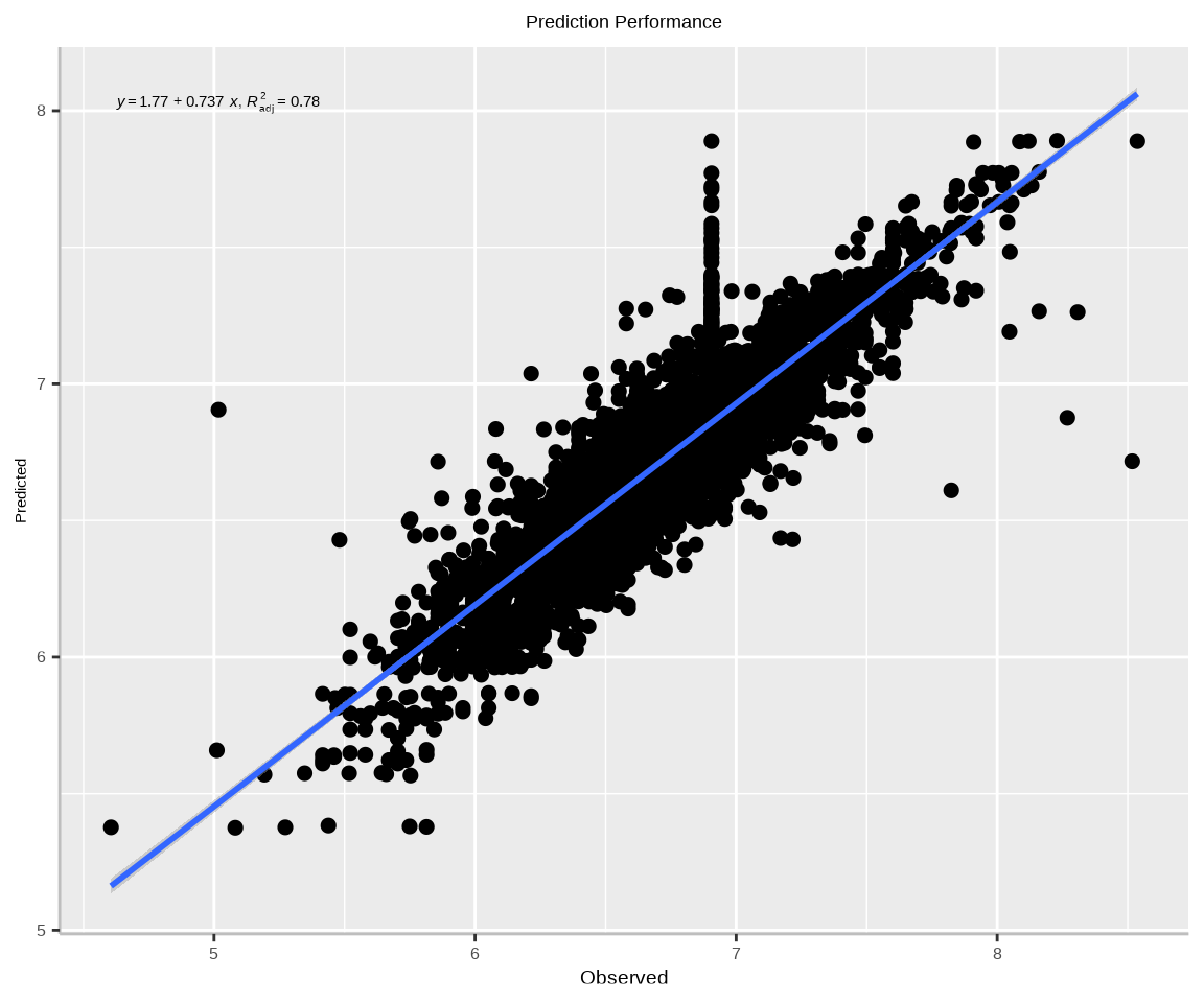
Predictions
The predict() function can be used to generate predictions from the fitted model. By specifying the argument type = "response", the function returns the predicted values on the original scale of the dependent variable.
Code
wages$predict<-predict(model.wb, type ="response", newdata = wages)head(wages$predict)
Registered S3 methods overwritten by 'ggpp':
  method                  from
  heightDetails.titleGrob ggplot2
  widthDetails.titleGrob  ggplot2
Attaching package: 'ggpp'
The following object is masked from 'package:ggplot2':

    annotate
Code
formula<-y~xggplot(wages.df, aes(x=lwage, y=predict)) +geom_point(size=2) +# draw fitted linegeom_smooth(method ="lm", formula = formula) +stat_poly_eq(use_label(c("eq", "adj.R2")), formula = formula) +# add plot titleggtitle("Prediction Performance") +theme(# center the plot titleplot.title =element_text(hjust =0.5),axis.line =element_line(colour ="gray"),# axis title font sizeaxis.title.x =element_text(size =14), # X and axis font sizeaxis.text.y=element_text(size=12,vjust =0.5, hjust=0.5),axis.text.x =element_text(size=12))+xlab("Observed") +ylab("Predicted")
Simulation
The simulate() function can be used to simulate data from the fitted model. By specifying the argument nsim = 1000, the function generates 1000 simulated datasets based on the model specifications.
   Min. 1st Qu.  Median    Mean 3rd Qu.    Max.
  6.044   6.759   6.791   6.728   6.810   6.877
Fit a “contextual” Model
To specify a model where occasion-level predictors do not have their means subtracted, use the argument model = "contextual." The term “contextual” refers to the interpretation of these variables when this option is selected.
Occasion Level Predictors: These predictors vary within units across different time points. For instance, in a panel data set, a variable like union membership may change over various years for the same individual.
Mean Subtracted: In some panel models, occasion-level predictors are mean-centered, meaning that the mean value of the predictor is subtracted from each observation. This isolates the within-unit variation.
Contextual Specification: If you prefer the model to use the raw values of the occasion-level predictors without mean subtraction, you can specify model = "contextual." This indicates that the predictors will be interpreted in their original scale and context.
By using the model = "contextual" argument, the model asserts that occasion-level predictors (e.g., lag(union)) will not have their means subtracted. Consequently, these predictors are interpreted in their original context, offering a “contextual” understanding of their effects on the dependent variable.
MODEL INFO:
Entities: 595
Time periods: 2-7
Dependent variable: lwage
Model type: Linear mixed effects
Specification: contextual

MODEL FIT:
AIC = 1387.25, BIC = 1449.06
Pseudo-R² (fixed effects) = 0.13
Pseudo-R² (total) = 0.74
Entity ICC = 0.7

WITHIN EFFECTS:
---------------------------------------------------------
                    Est.   S.E.   t val.      d.f.      p
---------------- ------- ------ -------- --------- ------
lag(union)          0.05   0.03     1.95   3034.28   0.05
wks                -0.00   0.00    -1.55   2993.12   0.12
---------------------------------------------------------

CONTEXTUAL EFFECTS:
----------------------------------------------------------------
                           Est.   S.E.   t val.      d.f.      p
----------------------- ------- ------ -------- --------- ------
(Intercept)                6.62   0.23    28.54    591.57   0.00
imean(lag(union))         -0.08   0.04    -1.96   1292.37   0.05
imean(wks)                 0.01   0.00     1.15    649.11   0.25
blk                       -0.26   0.07    -3.73    803.10   0.00
fem                       -0.44   0.05    -8.87    587.69   0.00
----------------------------------------------------------------

CROSS-LEVEL INTERACTIONS:
------------------------------------------------------------
                       Est.   S.E.   t val.      d.f.      p
-------------------- ------ ------ -------- --------- ------
lag(union):blk         0.08   0.09     0.91   1906.99   0.36
------------------------------------------------------------

p values calculated using Satterthwaite d.f.

RANDOM EFFECTS:
------------------------------------
  Group      Parameter    Std. Dev.
---------- ------------- -----------
    id      (Intercept)    0.3533
 Residual                  0.2327
------------------------------------
Fit a “between” or Random Effect Model
If we want the model specified such that the occasion level predictors do, You may also use model = “between” to fit what is known as the random effects model, which does not disaggregate the within- and between-entity variation. To effectively specify the model while taking into account the occasion-level predictors, we can utilize the option model = "between." This approach aligns with what econometricians refer to as the random effects model. Unlike fixed effects models, the random effects model does not distinguish between variations that occur within individual entities—such as repeated measures over time—and those that occur between different entities. By employing this model, we can analyze data that captures both the overall trends across different groups and the inherent differences among those groups, providing a comprehensive understanding of the underlying patterns.
MODEL INFO:
Entities: 595
Time periods: 2-7
Dependent variable: lwage
Model type: Linear mixed effects
Specification: between

MODEL FIT:
AIC = 1376.58, BIC = 1426.02
Pseudo-R² (fixed effects) = 0.13
Pseudo-R² (total) = 0.74
Entity ICC = 0.7

BETWEEN EFFECTS:
----------------------------------------------------------
                     Est.   S.E.   t val.      d.f.      p
----------------- ------- ------ -------- --------- ------
(Intercept)          6.85   0.05   128.54   3547.62   0.00
lag(union)           0.02   0.02     0.76   2865.05   0.45
wks                 -0.00   0.00    -1.25   3249.08   0.21
blk                 -0.27   0.07    -3.79    801.21   0.00
fem                 -0.44   0.05    -8.95    593.56   0.00
----------------------------------------------------------

CROSS-LEVEL INTERACTIONS:
------------------------------------------------------------
                       Est.   S.E.   t val.      d.f.      p
-------------------- ------ ------ -------- --------- ------
lag(union):blk         0.07   0.09     0.82   1897.19   0.41
------------------------------------------------------------

p values calculated using Satterthwaite d.f.

RANDOM EFFECTS:
------------------------------------
  Group      Parameter    Std. Dev.
---------- ------------- -----------
    id      (Intercept)    0.3544
 Residual                  0.2328
------------------------------------
Panel Regression Models with Generalized Estimating Equations (GEE)
GEE is a population-averaged approach for analyzing panel (longitudinal) data that accounts for within-cluster correlation (e.g., repeated measurements within individuals, firms, or households). Unlike mixed-effects models, GEE does not model individual-specific random effects but instead uses a working correlation structure to adjust standard errors and coefficients for dependency in the data. Here’s how to use GEE for panel regression:
Key Features of GEE are below:
Population-Averaged Effects: Estimates marginal (average) effects across the population.
Robustness: Provides valid inference even if the correlation structure is misspecified (due to robust “sandwich” standard errors).
Flexible Correlation Structures:
Independence: No correlation (equivalent to pooled OLS)
Exchangeable: Constant correlation across time (e.g., \(cor(y_it, y_is) = ρ\)).
AR(1): Correlation declines with time lag (e.g., \(cor(y_it, y_i(t-1)) = ρ\)).
Unstructured: No constraints on correlation patterns.
When to Use GEE?
Population-Averaged Inference: When interest lies in average effects (e.g., policy impacts across a population).
Robustness to Correlation Misspecification: When the true correlation structure is unknown.
Large Clusters: Requires many clusters (e.g., ≥ 30) for reliable standard errors.
GEE vs. Mixed-Effects Models
Aspect
GEE
Mixed-Effects Models
Inference
Population-averaged
Subject-specific
Correlation
Working correlation (adjusted)
Explicitly modeled (random effects)
Efficiency
Less efficient if RE is correct
More efficient if RE is correct
Assumptions
Robust to correlation misspec.
Requires correct random effects spec.
Fit a Linear GEE Model
We will WageData dataset to fit a GEE model using the wbgee() function from the {panelr} package.
Code
data("WageData", package ="panelr")wages <-panel_data(WageData, id = id, wave = t)
The model aims to explain the log of wages (lwage) based on several independent variables and their interactions:
MODEL INFO:
Entities: 595
Time periods: 2-7
Dependent variable: lwage
Model type: Linear GEE
Variance: ar1 (alpha = 0.85)
Specification: within-between

MODEL FIT:
QIC = 655.54, QICu = 653.36, CIC = 9.09

WITHIN EFFECTS:
-----------------------------------------------
                    Est.   S.E.   z val.      p
---------------- ------- ------ -------- ------
lag(union)          0.02   0.02     0.98   0.33
wks                -0.00   0.00    -0.82   0.41
-----------------------------------------------

BETWEEN EFFECTS:
------------------------------------------------------
                           Est.   S.E.   z val.      p
----------------------- ------- ------ -------- ------
(Intercept)                6.61   0.24    27.12   0.00
imean(lag(union))         -0.01   0.03    -0.40   0.69
imean(wks)                 0.00   0.01     0.75   0.45
blk                       -0.23   0.06    -3.86   0.00
fem                       -0.43   0.05    -8.94   0.00
------------------------------------------------------

CROSS-LEVEL INTERACTIONS:
---------------------------------------------------
                        Est.   S.E.   z val.      p
-------------------- ------- ------ -------- ------
lag(union):blk         -0.11   0.05    -2.22   0.03
---------------------------------------------------
First Differences Models using GLS
First differences models are a common approach to analyzing panel data when the focus is on the change in the dependent variable and the independent variables over time. The fdm() function in the panelr package estimates first differences models using Generalized Least Squares (GLS) estimation. This method is useful for examining the impact of time-varying predictors on the change in the dependent variable while controlling for individual-specific effects.
Fit a First Differences Model
The code below fits a first differences model using the fdm() function from the {panelr} package. The model aims to explain the change in the log of wages (lwage) based on the change in the number of weeks worked (wks) and the change in union membership (union).
Code
model.fdm <-fdm(lwage ~ wks + union, data = wages)summary(model.fdm)
MODEL INFO:
Entities: 595
Time periods: 2-7
Dependent variable: lwage
Variance structure: toeplitz-1 (theta = -0.44)

MODEL FIT:
AIC = -2500.35, BIC = -2469.45

Standard errors: CR2
-----------------------------------------------
                    Est.   S.E.   t val.      p
----------------- ------ ------ -------- ------
(Intercept)         0.10   0.00    54.86   0.00
wks                 0.00   0.00     0.47   0.64
union               0.02   0.02     0.90   0.37
-----------------------------------------------
The output of the summary() function provides the coefficients, standard errors, t-values, and p-values for the model parameters. The fdm() function estimates the first differences model using GLS estimation, which accounts for individual-specific effects and time-varying predictors. The model results include the estimated coefficients for the change in the number of weeks worked (wks) and the change in union membership (union).
Asymmetric Effects Models using First Differences
Asymmetric effects models are a type of panel regression model that allows for different effects of predictors on the dependent variable depending on the direction of change. The asym() function in the panelr package estimates asymmetric effects models using first differences. This method is useful for examining how predictors affect the dependent variable differently when they increase or decrease.
Fit an Asymmetric Effects Model
The code below fits an asymmetric effects model using the asym() function from the {panelr} package. The model aims to explain the change in the log of wages (lwage) based on the change in the number of weeks worked (wks) and the change in union membership (union), with different effects for positive and negative changes in the predictors.
Code
model.asym <-asym(lwage ~ wks + union, data = wages)summary(model.asym)
MODEL INFO:
Entities: 595
Time periods: 2-7
Dependent variable: lwage
Model type: Linear asymmetric effects (first differences)
Variance structure: toeplitz-1 (theta = -0.44)

Standard errors: Cluster-robust (CR2)
------------------------------------------------
                     Est.   S.E.   t val.      p
----------------- ------- ------ -------- ------
(Intercept)          0.10   0.00    43.17   0.00
+wks                 0.00   0.00     0.50   0.62
-wks                -0.00   0.00    -0.30   0.76
+union               0.01   0.02     0.53   0.60
-union              -0.03   0.03    -0.97   0.33
------------------------------------------------

Tests of asymmetric effects:
--------------------------
              chi^2      p
----------- ------- ------
wks            0.01   0.94
union          0.39   0.53
--------------------------
The output of the summary() function provides the coefficients, standard errors, t-values, and p-values for the model parameters. The asym() function estimates the asymmetric effects model using first differences, which allows for different effects of the predictors on the dependent variable depending on the direction of change. The model results include the estimated coefficients for the change in the number of weeks worked (wks) and the change in union membership (union), with separate effects for positive and negative changes.
Asymmetric Effects Models using GEE
The asym_gee() function in the panelr package estimates asymmetric effects models using Generalized Estimating Equations (GEE). This method is useful for analyzing panel data with repeated measurements and examining how predictors affect the dependent variable differently depending on the direction of change. The asym_gee() function allows for flexible correlation structures and robust standard errors in the estimation of asymmetric effects models.
Fit an Asymmetric Effects Model with GEE
The code below fits an asymmetric effects model using the asym_gee() function from the {panelr} package. The model aims to explain the log of wages (lwage) based on the number of weeks worked (wks) and union membership (union), with different effects for positive and negative changes in the predictors.
Code
model.asym_gee <-asym_gee(lwage ~ wks + union, data = wages)summary(model.asym_gee)
MODEL INFO:
Entities: 595
Time periods: 2-7
Dependent variable: lwage
Model family: Linear
Variance: ar1 (alpha = -0.31)
Specification: Asymmetric effects (via GEE)

MODEL FIT:
QIC = 134.36, QICu = 128.04, CIC = 8.16

------------------------------------------------
                     Est.   S.E.   z val.      p
----------------- ------- ------ -------- ------
(Intercept)          0.10   0.00    43.07   0.00
+wks                 0.00   0.00     0.26   0.80
-wks                -0.00   0.00    -0.14   0.89
+union               0.01   0.02     0.36   0.72
-union              -0.03   0.03    -0.93   0.35
------------------------------------------------

Tests of asymmetric effects:
--------------------------
              chi^2      p
----------- ------- ------
wks            0.00   0.96
union          0.45   0.50
--------------------------
Summary and Conclusions
This tutorial provided an overview of panel regression models fit via the panelr package in R. Panel data analysis involves repeated measurements of the same units over multiple time periods, and panel regression models are used to analyze the relationships between variables in panel data. The panelr package provides functions for data preparation, modeling, and interpretation of panel data, making it easier to work with longitudinal datasets. The wbm() function fits panel regression models using multilevel modeling, while the wbgee() function fits models with Generalized Estimating Equations (GEE). The fdm() function estimates first differences models, and the asym() and asym_gee() functions fit asymmetric effects models using first differences and GEE, respectively. These functions offer a flexible and user-friendly approach to analyzing panel data and estimating regression models with different specifications. By using the panelr package, researchers can conduct panel data analysis more efficiently and effectively, gaining insights into the dynamics of longitudinal datasets.