5. S-shaped Functions or Sigmoid Models

An S-shaped or sigmoid function is a mathematical function that produces a characteristic “S” shaped curve. This type of function is used in various fields such as machine learning, neural networks, and statistics due to its property of mapping any real-valued number into a value between 0 and 1.

The most commonly used sigmoid function is the logistic function, defined as:

\[ \sigma(x) = \frac{1}{1 + e^{-x}} \]

where:

$\sigma(x)$ is the output of the sigmoid function.
$x$ is the input to the function.
$e# is the base of the natural logarithm, approximately equal to 2.71828.

The logistic function has several important properties:

Range: The output of the logistic function is always between 0 and 1.
Saturation: As the input $x$ becomes very large positively, the output approaches 1. As $x$ becomes very large negatively, the output approaches 0.
Symmetry: The logistic function is symmetric around $x = 0$.
Derivative: The derivative of the logistic function can be expressed in terms of the function itself:

\[ \sigma'(x) = \sigma(x) (1 - \sigma(x)) \]

Applications:

Neural Networks: Sigmoid functions are used as activation functions in neural networks, helping to introduce non-linearity into the model.
Logistic Regression: In logistic regression, the sigmoid function is used to model the probability that a given input belongs to a particular class.
Biology: Sigmoid curves are often used to model population growth, enzyme kinetics, and dose-response relationships.

The sigmoid function’s ability to map any real-valued number to a value between 0 and 1 makes it particularly useful in scenarios where probabilities or binary outcomes are modeled. By adjusting the parameters of the function, it can be used to represent a wide range of relationships between variables. We can use the sigmoid function to model the growth of a population over time, the response of an enzyme to substrate concentration, or the probability of an event occurring based on certain features.

Fit S-shaped Models in R

In this tutorial, we will explore how to fit and visualize S-shaped functions in R. S-shaped functions, also known as sigmoid functions, are mathematical functions that exhibit an S-shaped curve. These functions are commonly used in various fields such as biology, economics, and machine learning to model growth, decay, and other processes that exhibit a characteristic S-shaped pattern.

Install Required R Packages

Code

# Packages List
packages <- c(
  "tidyverse",   # Includes readr, dplyr, ggplot2, etc.
  'patchwork',   # for visualization
  'minpack.lm',  # for damped exponential model
  'nlstools',    # for bootstrapping
  'nls2',        # for fitting multiple models
  'broom',       # for tidying model output
  'nlsr',        # for constrained optimization
  'drc',         # for dose-response models
  'growthrates'  # for growth models
)

#| warning: false
#| error: false

# Install missing packages
new_packages <- packages[!(packages %in% installed.packages()[,"Package"])]
if(length(new_packages)) install.packages(new_packages)

# Verify installation
cat("Installed packages:\n")
print(sapply(packages, requireNamespace, quietly = TRUE))

Load R Packages

Code

# Load packages with suppressed messages
invisible(lapply(packages, function(pkg) {
  suppressPackageStartupMessages(library(pkg, character.only = TRUE))
}))

Code

# Check loaded packages
cat("Successfully loaded packages:\n")

Successfully loaded packages:

Code

print(search()[grepl("package:", search())])

 [1] "package:growthrates" "package:deSolve"     "package:lattice"    
 [4] "package:drc"         "package:MASS"        "package:nlsr"       
 [7] "package:broom"       "package:nls2"        "package:proto"      
[10] "package:nlstools"    "package:minpack.lm"  "package:patchwork"  
[13] "package:lubridate"   "package:forcats"     "package:stringr"    
[16] "package:dplyr"       "package:purrr"       "package:readr"      
[19] "package:tidyr"       "package:tibble"      "package:ggplot2"    
[22] "package:tidyverse"   "package:stats"       "package:graphics"   
[25] "package:grDevices"   "package:utils"       "package:datasets"   
[28] "package:methods"     "package:base"

S-shaped Functions in R

Here, we will demonstrate how to fit and plot the sigmoid function in R:

Code

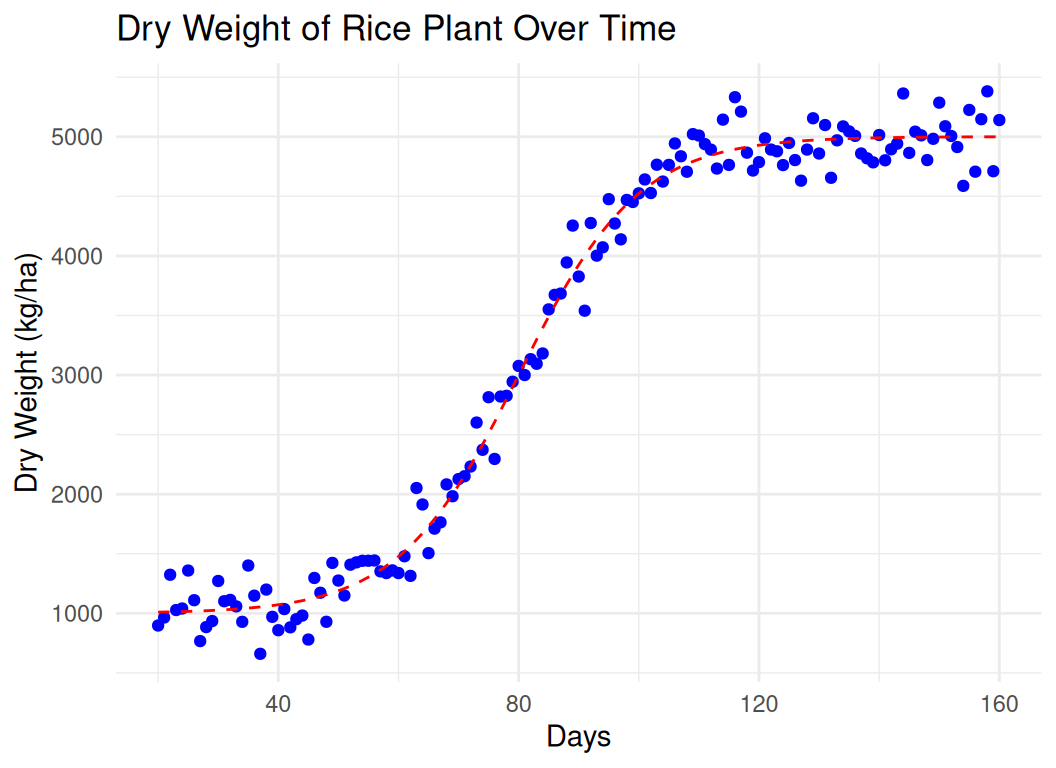
# Set seed for reproducibility
set.seed(123)

# Generate days vector from 20 to 160
days <- 20:160

# Define the logistic growth function
logistic_growth <- function(x, L, k, x0) {
  L / (1 + exp(-k * (x - x0)))
}

# Parameters for the logistic function
L <- 5000  # maximum dry weight (kg/ha)
k <- 0.1   # growth rate
x0 <- 80   # mid-point of the growth

# Generate the dry weight values using the logistic growth function
dry_weight <- logistic_growth(days, L, k, x0)

# Adjust the minimum value to be 1000 kg/ha
dry_weight <- dry_weight * (4000 / max(dry_weight)) + 1000

# Add noise to the dry weight values
noise <- rnorm(length(dry_weight), mean = 0, sd = 200)
dry_weight_noisy <- dry_weight + noise

# Create a data frame
data <- data.frame(Days = days, DryWeight = dry_weight_noisy)

# Plot the data
ggplot(data, aes(x = Days, y = DryWeight)) +
  geom_point(color = "blue") +
  geom_line(aes(y = logistic_growth(Days, L, k, x0) * (4000 / max(logistic_growth(Days, L, k, x0))) + 1000), color = "red", linetype = "dashed") +
  labs(title = "Dry Weight of Rice Plant Over Time",
       x = "Days",
       y = "Dry Weight (kg/ha)") +
  theme_minimal()

Two-Parameter Logistic Function

The two-parameter logistic function is a simplified version of the logistic function with two parameters: the growth rate and the midpoint.

\[ f(x) = \frac{1}{1 + e^{-k(x - x_0)}} \]

where: - $k$ is the growth rate. - $x_0$ is the midpoint of the curve.

Below step-by-step implementation of *2-parameter logistic in R

Define the 2PL Function

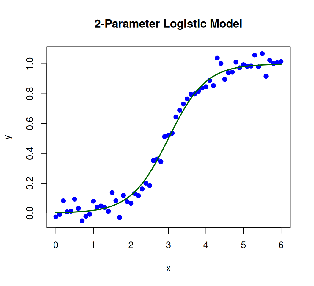
The 2-parameter logistic (2PL) function is an S-shaped curve defined by two parameters:
- a (slope/discrimination parameter, controlling steepness)
- b (location/difficulty parameter, midpoint where the response is 0.5).

Code

logistic_2pl <- function(x, a, b) {
  1 / (1 + exp(-a * (x - b)))
}

Generate Synthetic Data

Code

set.seed(123)
a_true <- 2   # True slope parameter
b_true <- 3   # True midpoint parameter
x <- seq(0, 6, by = 0.1)
y <- logistic_2pl(x, a_true, b_true) + rnorm(length(x), sd = 0.05)  # Add noise
# plot the data
plot(x, y, pch = 19, col = "blue", main = "2-Parameter Logistic Model", xlab = "x", ylab = "y")
curve(logistic_2pl(x, a_true, b_true), add = TRUE, lwd = 2, col = "darkgreen")  # True curve

Fit the Model Using Nonlinear Least Squares (`nls`)

Code

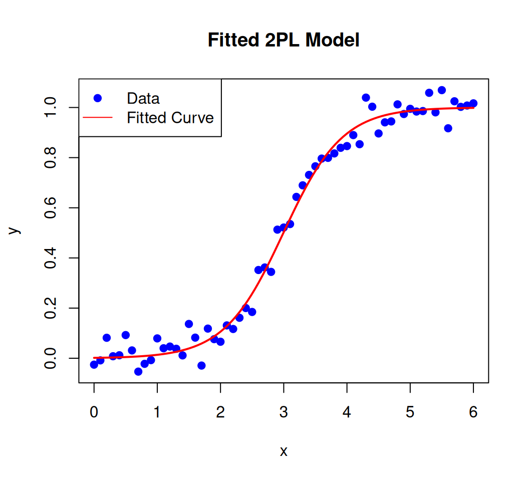
fit <- nls(y ~ 1 / (1 + exp(-a * (x - b))), 
          start = list(a = 1, b = 2))  # Provide reasonable starting guesses
summary(fit)  # View estimated parameters


Formula: y ~ 1/(1 + exp(-a * (x - b)))

Parameters:
  Estimate Std. Error t value Pr(>|t|)    
a  2.14324    0.09593   22.34   <2e-16 ***
b  2.99463    0.02371  126.29   <2e-16 ***
---
Signif. codes:  0 '***' 0.001 '**' 0.01 '*' 0.05 '.' 0.1 ' ' 1

Residual standard error: 0.04482 on 59 degrees of freedom

Number of iterations to convergence: 7 
Achieved convergence tolerance: 2.641e-06

Plot the Fitted Curve

Code

x_pred <- seq(min(x), max(x), length.out = 100)
y_pred <- predict(fit, newdata = data.frame(x = x_pred))

plot(x, y, pch = 19, col = "blue", main = "Fitted 2PL Model", xlab = "x", ylab = "y")
lines(x_pred, y_pred, col = "red", lwd = 2)
legend("topleft", legend = c("Data", "Fitted Curve"), 
       col = c("blue", "red"), pch = c(19, NA), lty = c(NA, 1))

Three-Parameter Logistic Function

The three-parameter logistic function adds a third parameter to account for the asymptote.

\[ f(x) = \frac{A}{1 + e^{-k(x - x_0)}} \]

where: - $A$ is the maximum value (asymptote). - $k$ is the growth rate. - $x_0$ is the midpoint of the curve.

Define the 3PL Function

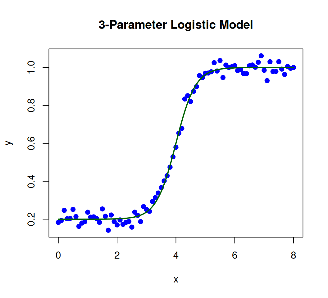
Parameters:
- a: Slope/discrimination (steepness)
- b: Location/difficulty (midpoint)
- c: Lower asymptote (baseline probability when ( x -))

Code

logistic_3pl <- function(x, a, b, c) {
  c + (1 - c) / (1 + exp(-a * (x - b)))
}

Generate Synthetic Data

Code

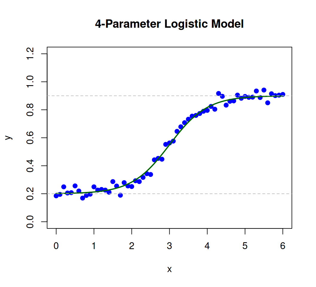
set.seed(123)
a_true <- 3    # True slope
b_true <- 4    # True midpoint
c_true <- 0.2  # True lower asymptote (e.g., 20% guessing probability)
x <- seq(0, 8, by = 0.1)
y <- logistic_3pl(x, a_true, b_true, c_true) + rnorm(length(x), sd = 0.03)  # Add noise
# plot the data
plot(x, y, pch = 19, col = "blue", main = "3-Parameter Logistic Model", xlab = "x", ylab = "y")
curve(logistic_3pl(x, a_true, b_true, c_true), add = TRUE, lwd = 2, col = "darkgreen")  # True curve

Fit the Model Using `nls`

Use bounds for parameter c (e.g., $0 \leq c \leq 1$):

Code

library(nlsr)  # For better handling of bounds (install if needed)
fit <- nls(y ~ c + (1 - c)/(1 + exp(-a * (x - b))), 
          start = list(a = 1, b = 2, c = 0.1), 
          lower = list(a = 0.1, b = -Inf, c = 0), 
          upper = list(a = Inf, b = Inf, c = 0.5), 
          algorithm = "port")  # Constrained optimization

summary(fit)  # View parameter estimates


Formula: y ~ c + (1 - c)/(1 + exp(-a * (x - b)))

Parameters:
  Estimate Std. Error t value Pr(>|t|)    
a  2.94569    0.12812   22.99   <2e-16 ***
b  3.99373    0.01707  234.00   <2e-16 ***
c  0.19976    0.00526   37.98   <2e-16 ***
---
Signif. codes:  0 '***' 0.001 '**' 0.01 '*' 0.05 '.' 0.1 ' ' 1

Residual standard error: 0.02784 on 78 degrees of freedom

Algorithm "port", convergence message: both X-convergence and relative convergence (5)

Plot the Fitted Curve

Code

x_pred <- seq(min(x), max(x), length.out = 100)
y_pred <- predict(fit, newdata = data.frame(x = x_pred))

plot(x, y, pch = 19, col = "blue", main = "Fitted 3PL Model", xlab = "x", ylab = "y")
lines(x_pred, y_pred, col = "red", lwd = 2)
abline(h = coef(fit)["c"], lty = 2, col = "gray")  # Plot lower asymptote
legend("topleft", legend = c("Data", "Fitted Curve", "Lower Asymptote (c)"), 
       col = c("blue", "red", "gray"), pch = c(19, NA, NA), lty = c(NA, 1, 2))

Four-Parameter Logistic Function $$

The four-parameter logistic function includes an additional parameter to adjust the minimum value.

\[ f(x) = A + \frac{(B - A)}{1 + e^{-k(x - x_0)}} \]

where: - $A$ is the minimum value (lower asymptote). - $B$ is the maximum value (upper asymptote). - $k$ is the growth rate. - $x_0$ is the midpoint of the curve.

Define the 4PL Function

The 4-parameter logistic (4PL) function extends the 3PL model by adding an upper asymptote parameter (d), allowing the curve to approach a value other than 1. It is widely used in dose-response studies, bioassays, and growth modeling. The formula is:

Code

logistic_4pl <- function(x, a, b, c, d) {
  c + (d - c) / (1 + exp(-a * (x - b)))
}

Generate Synthetic Data

Code

set.seed(123)
a_true <- 2    # True slope
b_true <- 3    # True midpoint
c_true <- 0.2  # True lower asymptote
d_true <- 0.9  # True upper asymptote (not 1!)
x <- seq(0, 6, by = 0.1)
y <- logistic_4pl(x, a_true, b_true, c_true, d_true) + rnorm(length(x), sd = 0.03)  # Add noise
# plot the data
plot(x, y, pch = 19, col = "blue", main = "4-Parameter Logistic Model", 
     xlab = "x", ylab = "y", ylim = c(0, 1.2))
curve(logistic_4pl(x, a_true, b_true, c_true, d_true), add = TRUE, lwd = 2, col = "darkgreen")  # True curve
abline(h = c(c_true, d_true), lty = 2, col = "gray")  # Plot asymptotes

Fit the Model

Option 1: Using `nls` (Nonlinear Least Squares)

Use constraints for $c$ and $d$ (e.g., $ 0 c d $):

Code

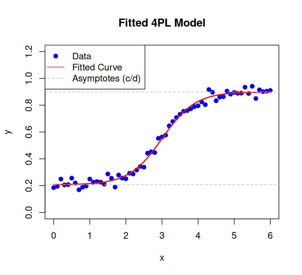
# Provide reasonable starting guesses (critical for convergence)
fit <- nls(y ~ c + (d - c)/(1 + exp(-a * (x - b))), 
          start = list(a = 1, b = 3, c = 0.1, d = 0.8), 
          lower = list(a = 0.1, b = -Inf, c = 0, d = 0.5), 
          upper = list(a = 5, b = Inf, c = 0.3, d = 1), 
          algorithm = "port")  # Use "port" algorithm for bounds

summary(fit)  # View parameter estimates


Formula: y ~ c + (d - c)/(1 + exp(-a * (x - b)))

Parameters:
  Estimate Std. Error t value Pr(>|t|)    
a 2.178090   0.119456   18.23   <2e-16 ***
b 3.006462   0.027759  108.31   <2e-16 ***
c 0.206874   0.007416   27.89   <2e-16 ***
d 0.898834   0.007449  120.66   <2e-16 ***
---
Signif. codes:  0 '***' 0.001 '**' 0.01 '*' 0.05 '.' 0.1 ' ' 1

Residual standard error: 0.02716 on 57 degrees of freedom

Algorithm "port", convergence message: relative convergence (4)

Option 2: Using the `drc` Package

The drc package provides a more straightforward interface for fitting dose-response models, including the 4PL model.

Code

fit_drc <- drm(y ~ x, data = data.frame(x, y), 
              fct = L.4(fixed = c(NA, NA, NA, NA)))  # 4PL model
summary(fit_drc)  # Clean output with parameter names: b, c, d, e (slope, lower, upper, midpoint)


Model fitted: Logistic (ED50 as parameter) (4 parms)

Parameter estimates:

                Estimate Std. Error t-value   p-value    
b:(Intercept) -2.1781753  0.1230503 -17.701 < 2.2e-16 ***
c:(Intercept)  0.2068784  0.0073609  28.105 < 2.2e-16 ***
d:(Intercept)  0.8988279  0.0076342 117.736 < 2.2e-16 ***
e:(Intercept)  3.0064585  0.0277626 108.291 < 2.2e-16 ***
---
Signif. codes:  0 '***' 0.001 '**' 0.01 '*' 0.05 '.' 0.1 ' ' 1

Residual standard error:

 0.02715902 (57 degrees of freedom)

Plot the Fitted Curve

Code

x_pred <- seq(min(x), max(x), length.out = 100)
y_pred <- predict(fit, newdata = data.frame(x = x_pred))  # For `nls` output
# OR: y_pred <- predict(fit_drc, newdata = data.frame(x = x_pred))  # For `drc` output

plot(x, y, pch = 19, col = "blue", main = "Fitted 4PL Model", 
     xlab = "x", ylab = "y", ylim = c(0, 1.2))
lines(x_pred, y_pred, col = "red", lwd = 2)
abline(h = c(coef(fit)[["c"]], coef(fit)[["d"]]), lty = 2, col = "gray")  # Fitted asymptotes
legend("topleft", legend = c("Data", "Fitted Curve", "Asymptotes (c/d)"), 
       col = c("blue", "red", "gray"), pch = c(19, NA, NA), lty = c(NA, 1, 2))

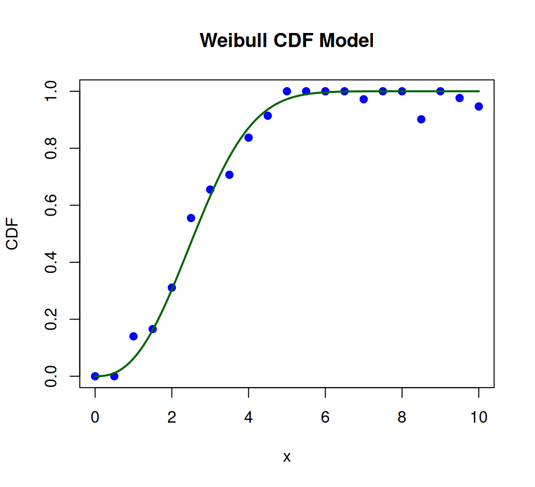
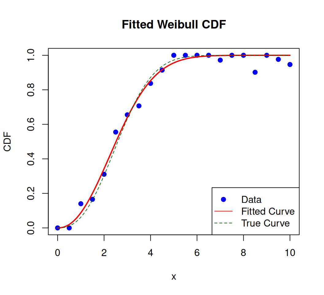
Weibull Function

The Weibull function is commonly used to model the distribution of lifetimes of products or components, where the probability of failure increases over time. It can also be used to model other phenomena where the rate of change is not constant. The Weibull function is a versatile model used in survival analysis, reliability engineering, and dose-response studies. Its cumulative distribution function (CDF) is S-shaped and defined by two parameters:

Shape (k): Controls the steepness and direction of the curve.
- $k < 1$: Decreasing hazard rate (e.g., early failures).
- $k = 1$: Exponential distribution (constant hazard rate).
- $k > 1$: Increasing hazard rate (e.g., wear-out failures).
Scale (λ): Determines the spread of the distribution (larger λ = wider spread).

The Weibull CDF is:

\[ f(x) = 1 - e^{-(x/\lambda)^k} \] ### Define the Weibull Function (CDF)

Code

weibull_cdf <- function(x, k, lambda) {
  1 - exp(-(x / lambda)^k)
}

Generate Synthetic Data

Code

set.seed(123)
k_true <- 2.5    # True shape parameter
lambda_true <- 3 # True scale parameter
x <- seq(0, 10, by = 0.5)
y <- weibull_cdf(x, k_true, lambda_true) + rnorm(length(x), sd = 0.05)  # Add noise
y <- pmax(pmin(y, 1), 0)  # Clip values between 0 and 1

Plot the Data

Code

plot(x, y, pch = 19, col = "blue", main = "Weibull CDF Model", xlab = "x", ylab = "CDF")
curve(weibull_cdf(x, k_true, lambda_true), add = TRUE, lwd = 2, col = "darkgreen")  # True curve

Fit the Model

Option 1: Nonlinear Least Squares (`nls`)

Code

fit_nls <- nls(y ~ 1 - exp(-(x / lambda)^k),
              start = list(k = 1, lambda = 5),  # Critical starting guesses
              lower = list(k = 0.1, lambda = 0.1),
              upper = list(k = 10, lambda = 10),
              algorithm = "port")  # Use "port" for bounds

summary(fit_nls)  # Estimated parameters


Formula: y ~ 1 - exp(-(x/lambda)^k)

Parameters:
       Estimate Std. Error t value Pr(>|t|)    
k       2.19027    0.15028   14.57 9.12e-12 ***
lambda  2.97249    0.06591   45.10  < 2e-16 ***
---
Signif. codes:  0 '***' 0.001 '**' 0.01 '*' 0.05 '.' 0.1 ' ' 1

Residual standard error: 0.03878 on 19 degrees of freedom

Algorithm "port", convergence message: relative convergence (4)

Option 2: Using the `drc` Package

Code

fit_drc <- drm(y ~ x, data = data.frame(x, y), 
              fct = W2.2())  # 2-parameter Weibull (shape = b, scale = e)
summary(fit_drc)  # Parameters: b (shape), d (fixed at 1), e (scale)


Model fitted: Weibull (type 2) with lower limit at 0 and upper limit at 1 (2 parms)

Parameter estimates:

              Estimate Std. Error t-value   p-value    
b:(Intercept) 2.190229   0.146402  14.960 5.766e-12 ***
e:(Intercept) 2.972499   0.065634  45.289 < 2.2e-16 ***
---
Signif. codes:  0 '***' 0.001 '**' 0.01 '*' 0.05 '.' 0.1 ' ' 1

Residual standard error:

 0.03878208 (19 degrees of freedom)

Plot the Fitted Curve

Code

x_pred <- seq(min(x), max(x), length.out = 100)
y_pred_nls <- predict(fit_nls, newdata = data.frame(x = x_pred))
# OR: y_pred_drc <- predict(fit_drc, newdata = data.frame(x = x_pred))

plot(x, y, pch = 19, col = "blue", main = "Fitted Weibull CDF", xlab = "x", ylab = "CDF")
lines(x_pred, y_pred_nls, col = "red", lwd = 2)  # `nls` prediction
curve(weibull_cdf(x, k_true, lambda_true), add = TRUE, lty = 2, col = "darkgreen")  # True curve
legend("bottomright", legend = c("Data", "Fitted Curve", "True Curve"), 
       col = c("blue", "red", "darkgreen"), pch = c(19, NA, NA), lty = c(NA, 1, 2))

Gompertz Function

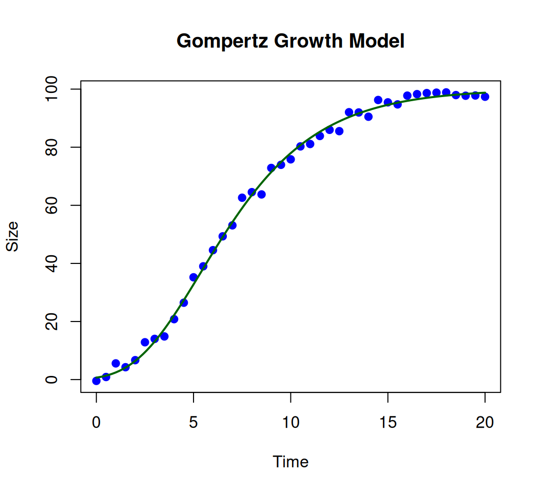
The Gompertz function is an asymmetric sigmoid curve used to model growth processes (e.g., tumor growth, population dynamics, or product adoption). It is defined by three parameters:

a: Upper asymptote (maximum value).
b: Displacement parameter (shifts the curve horizontally).
c: Growth rate (controls the steepness).

Its mathematical form is:
\[ f(x) = a \cdot e^{-b \cdot e^{-c \cdot x}} \]

Define the Gompertz Function

Code

gompertz <- function(x, a, b, c) {
  a * exp(-b * exp(-c * x))
}

Generate Synthetic Data

Code

set.seed(123)
a_true <- 100   # Upper asymptote
b_true <- 5     # Displacement parameter
c_true <- 0.3   # Growth rate
x <- seq(0, 20, by = 0.5)
y <- gompertz(x, a_true, b_true, c_true) + rnorm(length(x), sd = 2)  # Add noise

plot(x, y, pch = 19, col = "blue", main = "Gompertz Growth Model", xlab = "Time", ylab = "Size")
curve(gompertz(x, a_true, b_true, c_true), add = TRUE, lwd = 2, col = "darkgreen")  # True curve

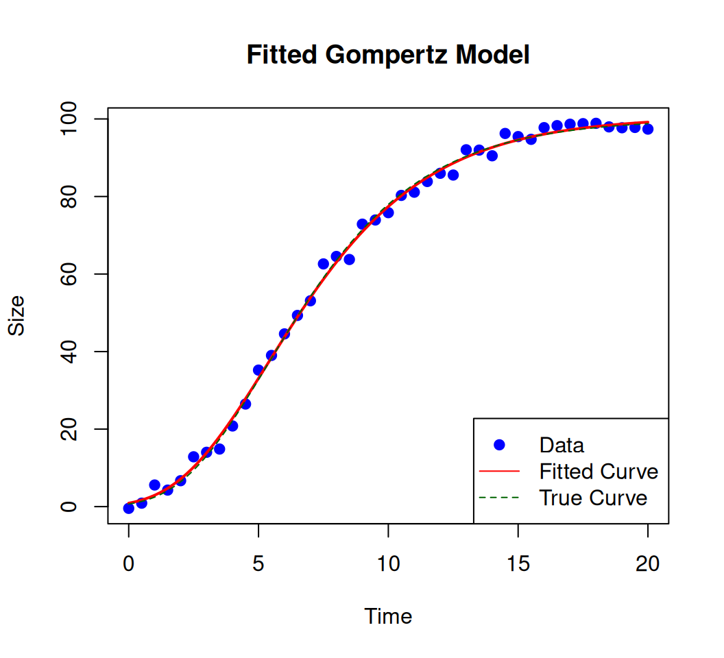
Fit the Model

Option 1: Nonlinear Least Squares (`nls`)

Code

fit_nls <- nls(y ~ a * exp(-b * exp(-c * x)),
              start = list(a = 90, b = 4, c = 0.2),  # Critical starting guesses
              control = nls.control(maxiter = 500))  # Increase iterations if needed
summary(fit_nls)


Formula: y ~ a * exp(-b * exp(-c * x))

Parameters:
   Estimate Std. Error t value Pr(>|t|)    
a 1.006e+02  7.033e-01  143.09   <2e-16 ***
b 4.714e+00  1.868e-01   25.23   <2e-16 ***
c 2.889e-01  7.356e-03   39.28   <2e-16 ***
---
Signif. codes:  0 '***' 0.001 '**' 0.01 '*' 0.05 '.' 0.1 ' ' 1

Residual standard error: 1.784 on 38 degrees of freedom

Number of iterations to convergence: 4 
Achieved convergence tolerance: 2.475e-06

Option 2: Using the `growthrates` Package

Code

fit_growth <- fit_growthmodel(FUN = grow_gompertz, 
                             p = c(y0 = 1, mumax = 0.3, K = 100),  # Parameters: initial size, growth rate, asymptote
                             time = x, 
                             y = y)
summary(fit_growth)


Parameters:
       Estimate Std. Error t value Pr(>|t|)    
y0    9.023e-01  1.720e-01   5.246 6.15e-06 ***
mumax 2.889e-01  7.356e-03  39.279  < 2e-16 ***
K     1.006e+02  7.033e-01 143.086  < 2e-16 ***
---
Signif. codes:  0 '***' 0.001 '**' 0.01 '*' 0.05 '.' 0.1 ' ' 1

Residual standard error: 1.784 on 38 degrees of freedom

Parameter correlation:
           y0   mumax       K
y0     1.0000 -0.9215  0.5571
mumax -0.9215  1.0000 -0.7480
K      0.5571 -0.7480  1.0000

Plot the Fitted Curve

Code

x_pred <- seq(min(x), max(x), length.out = 100)
y_pred <- predict(fit_nls, newdata = data.frame(x = x_pred))

plot(x, y, pch = 19, col = "blue", main = "Fitted Gompertz Model", xlab = "Time", ylab = "Size")
lines(x_pred, y_pred, col = "red", lwd = 2)  # Fitted curve
curve(gompertz(x, a_true, b_true, c_true), add = TRUE, lty = 2, col = "darkgreen")  # True curve
legend("bottomright", legend = c("Data", "Fitted Curve", "True Curve"), 
       col = c("blue", "red", "darkgreen"), pch = c(19, NA, NA), lty = c(NA, 1, 2))

Summary and Conclusion

This tutorial explored the implementation, fitting, and visualization of nonlinear functions in R, focusing on diffrenty types of S-shaped or sigmoid models. These models are usefull in various fields such as machine learning, neural networks, and statistics due to its property of mapping any real-valued number into a value between 0 and 1. By combining base R functions (nls, plot) with specialized packages (drc, growthrates), users can efficiently tackle complex modeling tasks. The workflow—defining equations, simulating data, fitting parameters, and validating results—equips researchers to analyze real-world phenomena, from drug efficacy to population dynamics. Future work could extend to hierarchical models, Bayesian fitting (e.g., brms), or machine learning hybrids for higher-dimensional data. The tutorial underscores R’s versatility as a tool for both exploratory and confirmatory nonlinear modeling.

References

Sigmoid function - Wikipedia
- Explanation of sigmoid functions and their characteristic S-shaped curve.
S-Shaped Curve - Fiveable
- Definition and explanations of S-shaped curves, often observed in natural and social phenomena.
S-shaped Functions - MetaSD
- Collection of small models using sigmoid functions with S-shaped characteristics.
Fit Sigmoidal Models - MathWorks
- Information on fitting sigmoidal models such as logistic and Gompertz functions.
S-shaped MF - MathWorks
- Description of S-shaped membership functions used in fuzzy logic.
V4L2 Device Sub-devices
- Documentation about sub-devices in V4L2, which might be useful for understanding complex device structures.

5. S-shaped Functions or Sigmoid Models

Fit S-shaped Models in R

Install Required R Packages

Load R Packages

S-shaped Functions in R

Two-Parameter Logistic Function

Define the 2PL Function

Generate Synthetic Data

Fit the Model Using Nonlinear Least Squares (nls)

Plot the Fitted Curve

Three-Parameter Logistic Function

Define the 3PL Function

Generate Synthetic Data

Fit the Model Using nls

Plot the Fitted Curve

Four-Parameter Logistic Function $$

Define the 4PL Function

Generate Synthetic Data

Fit the Model

Option 1: Using nls (Nonlinear Least Squares)

Option 2: Using the drc Package

Plot the Fitted Curve

Weibull Function

Generate Synthetic Data

Plot the Data

Fit the Model

Option 1: Nonlinear Least Squares (nls)

Option 2: Using the drc Package

Plot the Fitted Curve

Gompertz Function

Define the Gompertz Function

Generate Synthetic Data

Fit the Model

Option 1: Nonlinear Least Squares (nls)

Option 2: Using the growthrates Package

Plot the Fitted Curve

Summary and Conclusion

References

Fit the Model Using Nonlinear Least Squares (`nls`)

Fit the Model Using `nls`

Option 1: Using `nls` (Nonlinear Least Squares)

Option 2: Using the `drc` Package

Option 1: Nonlinear Least Squares (`nls`)

Option 2: Using the `drc` Package

Option 1: Nonlinear Least Squares (`nls`)

Option 2: Using the `growthrates` Package