6. Self-starting Function

Self-starting functions in R are special functions used in non-linear regression models that make the fitting process easier. These functions provide initial parameter estimates that help the fitting algorithm converge more efficiently. Non-linear models often require good starting values for the parameters, and self-starting functions automate this process.

Important Self-starting Functions

Self-starting functions in R automate the estimation of initial parameters for non-linear models, eliminating the need for manual specification. They are particularly useful in functions like nls() (non-linear least squares) where convergence heavily depends on starting values. Below are key self-starting functions, their descriptions, examples, and visualizations.

SSlogis: Self-starting logistic model.
SSfpl: Self-starting four-parameter logistic model.
SSweibull: Self-starting Weibull growth curve model.
SSgompertz: Self-starting Gompertz growth curve model.
SSasymp”: Self-starting asymptotic regression model.
SSmicmen: Self-starting Michaelis-Menten model.

Install Required R Packages

Code

# Packages List
packages <- c(
  "tidyverse",   # Includes readr, dplyr, ggplot2, etc.
  "nlme"       # For non-linear mixed-effects models
)

#| warning: false
#| error: false

# Install missing packages
new_packages <- packages[!(packages %in% installed.packages()[,"Package"])]
if(length(new_packages)) install.packages(new_packages)

# Verify installation
cat("Installed packages:\n")
print(sapply(packages, requireNamespace, quietly = TRUE))

Load R Packages

Code

# Load packages with suppressed messages
invisible(lapply(packages, function(pkg) {
  suppressPackageStartupMessages(library(pkg, character.only = TRUE))
}))

Code

# Check loaded packages
cat("Successfully loaded packages:\n")

Successfully loaded packages:

Code

print(search()[grepl("package:", search())])

 [1] "package:nlme"      "package:lubridate" "package:forcats"  
 [4] "package:stringr"   "package:dplyr"     "package:purrr"    
 [7] "package:readr"     "package:tidyr"     "package:tibble"   
[10] "package:ggplot2"   "package:tidyverse" "package:stats"    
[13] "package:graphics"  "package:grDevices" "package:utils"    
[16] "package:datasets"  "package:methods"   "package:base"

Logistic Growth Model: `SSlogis`

Model:

$y = $

Parameters:
- Asym: Asymptote (maximum value).
- xmid: x-value at the inflection point.
- scal: Scale parameter (inverse of the growth rate).

Code

   set.seed(123)
   x <- 1:20
   y <- SSlogis(x, Asym = 10, xmid = 10, scal = 3) + rnorm(20, sd = 0.5)
   df <- data.frame(x, y)
   
   fit <- nls(y ~ SSlogis(x, Asym, xmid, scal), data = df)
   summary(fit)


Formula: y ~ SSlogis(x, Asym, xmid, scal)

Parameters:
     Estimate Std. Error t value Pr(>|t|)    
Asym   9.9754     0.4016  24.842 8.43e-15 ***
xmid   9.8424     0.4084  24.098 1.39e-14 ***
scal   3.0210     0.3059   9.875 1.86e-08 ***
---
Signif. codes:  0 '***' 0.001 '**' 0.01 '*' 0.05 '.' 0.1 ' ' 1

Residual standard error: 0.5136 on 17 degrees of freedom

Number of iterations to convergence: 0 
Achieved convergence tolerance: 1.267e-06

Code

   # Predict and plot
   new_x <- data.frame(x = seq(1, 20, length.out = 100))
   new_y <- predict(fit, new_x)
   ggplot(df, aes(x, y)) +
     geom_point() +
     geom_line(data = data.frame(x = new_x$x, y = new_y), color = "red") +
     ggtitle("Logistic Model Fit with SSlogis")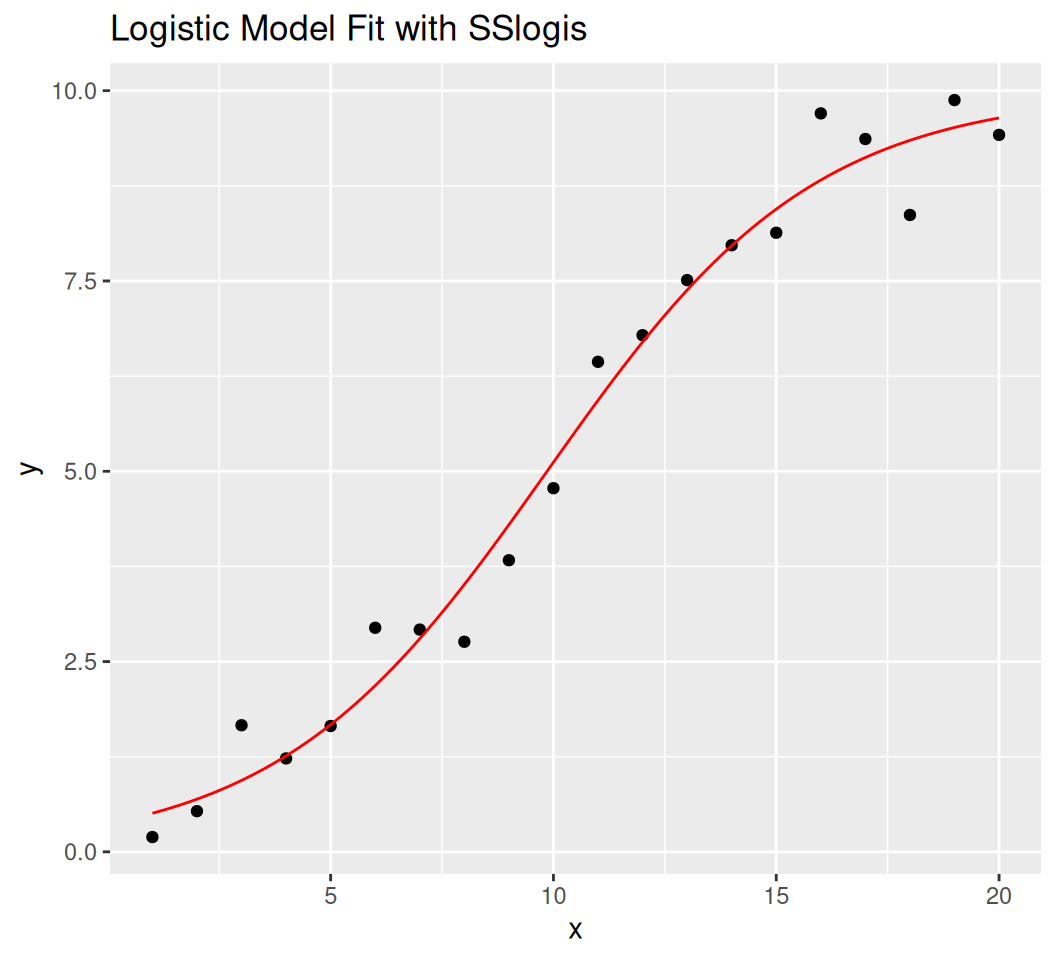

Four-Parameter Logistic Model: `SSfpl`

Model:

$y = A + \frac{B - A}{1 + (x/xmid)^scal}$
Parameters:
- A: Lower asymptote.
- B: Upper asymptote.
- xmid: x-value at the inflection point.
- scal: Slope parameter.

Code

set.seed(123)
x <- seq(0, 10, length.out = 50)
y <- SSfpl(x, A = 2, B = 10, xmid = 5, scal = 1) + rnorm(50, sd = 0.5)
df <- data.frame(x, y)

fit <- nls(y ~ SSfpl(x, A, B, xmid, scal), data = df)
summary(fit)


Formula: y ~ SSfpl(x, A, B, xmid, scal)

Parameters:
     Estimate Std. Error t value Pr(>|t|)    
A     2.27336    0.14283   15.92  < 2e-16 ***
B     9.94942    0.15096   65.91  < 2e-16 ***
xmid  5.12581    0.08473   60.50  < 2e-16 ***
scal  0.84530    0.07820   10.81 3.24e-14 ***
---
Signif. codes:  0 '***' 0.001 '**' 0.01 '*' 0.05 '.' 0.1 ' ' 1

Residual standard error: 0.4551 on 46 degrees of freedom

Number of iterations to convergence: 0 
Achieved convergence tolerance: 1.287e-06

Code

# Predict values for a smooth curve
new_x <- data.frame(x = seq(0, 10, length.out = 100))
pred_y <- predict(fit, newdata = new_x)

# Plot
ggplot(df, aes(x, y)) +
  geom_point(size = 2, alpha = 0.7) +
  geom_line(data = data.frame(x = new_x$x, y = pred_y), 
            color = "red", linewidth = 1) +
  labs(
    title = "Four-Parameter Logistic Model (SSfpl)",
    x = "x",
    y = "Response"
  ) +
  geom_hline(yintercept = coef(fit)["A"], linetype = "dashed", color = "blue") +
  geom_hline(yintercept = coef(fit)["B"], linetype = "dashed", color = "blue") +
  annotate("text", x = 1, y = coef(fit)["A"] + 0.5, 
           label = paste0("Lower Asym (A) = ", round(coef(fit)["A"], 2)), color = "blue") +
  annotate("text", x = 1, y = coef(fit)["B"] - 0.5, 
           label = paste0("Upper Asym (B) = ", round(coef(fit)["B"], 2)), color = "blue")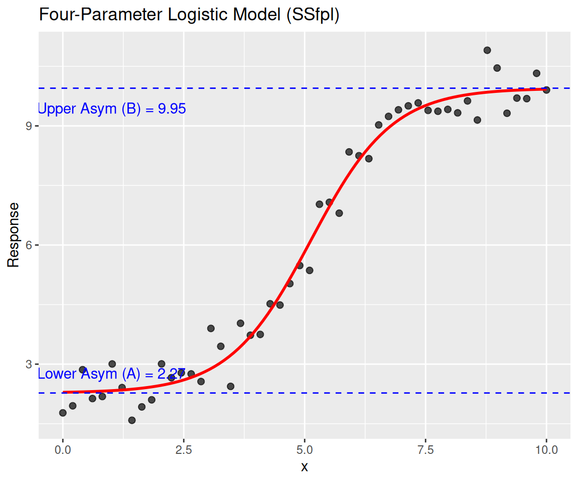

Weibull Growth Curve: `SSweibull`

Model:

$y = Asym - (Asym - Drop) e^{-exp((x - lrc) / pwr)}$
Parameters:
- Asym: Asymptote.
- Drop: Drop parameter.
- lrc: Natural logarithm of the rate constant.
- pwr: Power parameter.

Code

# Set seed for reproducibility
set.seed(123)

# Simulate Weibull growth data
x <- 1:30
y <- SSweibull(x, Asym = 100, Drop = 80, lrc = log(0.1), pwr = 2) + rnorm(30, sd = 3)
df <- data.frame(x, y)

# Fit Weibull model using self-starting function
weibull_fit <- nls(y ~ SSweibull(x, Asym, Drop, lrc, pwr), data = df)

# Model summary and parameters
summary(weibull_fit)


Formula: y ~ SSweibull(x, Asym, Drop, lrc, pwr)

Parameters:
     Estimate Std. Error t value Pr(>|t|)    
Asym  99.5733     0.6026 165.249  < 2e-16 ***
Drop  82.0570     6.3274  12.969 7.36e-13 ***
lrc   -2.2490     0.4594  -4.895 4.43e-05 ***
pwr    2.0591     0.3370   6.110 1.85e-06 ***
---
Signif. codes:  0 '***' 0.001 '**' 0.01 '*' 0.05 '.' 0.1 ' ' 1

Residual standard error: 2.964 on 26 degrees of freedom

Number of iterations to convergence: 0 
Achieved convergence tolerance: 8.536e-07

Code

cat("\nKey Parameters:",
    "\nUpper Asymptote (Asym):", coef(weibull_fit)["Asym"],
    "\nLower Asymptote:", coef(weibull_fit)["Asym"] - coef(weibull_fit)["Drop"],
    "\nRate Constant (exp(lrc)):", exp(coef(weibull_fit)["lrc"]),
    "\nPower Parameter:", coef(weibull_fit)["pwr"])


Key Parameters: 
Upper Asymptote (Asym): 99.57331 
Lower Asymptote: 17.51629 
Rate Constant (exp(lrc)): 0.1055008 
Power Parameter: 2.059132

Code

# Generate predictions for smooth curve
new_data <- data.frame(x = seq(1, 30, length.out = 300))
predicted <- predict(weibull_fit, newdata = new_data)

# Create visualization
ggplot(df, aes(x = x, y = y)) +
  geom_point(size = 2.5, alpha = 0.7, color = "darkblue") +
  geom_line(data = data.frame(x = new_data$x, y = predicted), 
            color = "red", linewidth = 1.2) +
  geom_hline(yintercept = coef(weibull_fit)["Asym"], 
             linetype = "dashed", color = "darkgreen") +
  geom_hline(yintercept = coef(weibull_fit)["Asym"] - coef(weibull_fit)["Drop"], 
             linetype = "dashed", color = "purple") +
  annotate("text", x = 5, y = coef(weibull_fit)["Asym"] + 5,
           label = paste("Upper Asymptote =", round(coef(weibull_fit)["Asym"], 1)),
           color = "darkgreen") +
  annotate("text", x = 5, y = (coef(weibull_fit)["Asym"] - coef(weibull_fit)["Drop"]) - 5,
           label = paste("Lower Asymptote =", 
                         round(coef(weibull_fit)["Asym"] - coef(weibull_fit)["Drop"], 1)),
           color = "purple") +
  labs(title = "Weibull Growth Curve Fit using SSweibull",
       subtitle = "Red: Fitted Curve | Dashed: Upper/Lower Asymptotes",
       x = "Time/Input Variable", 
       y = "Response") +
  theme_minimal()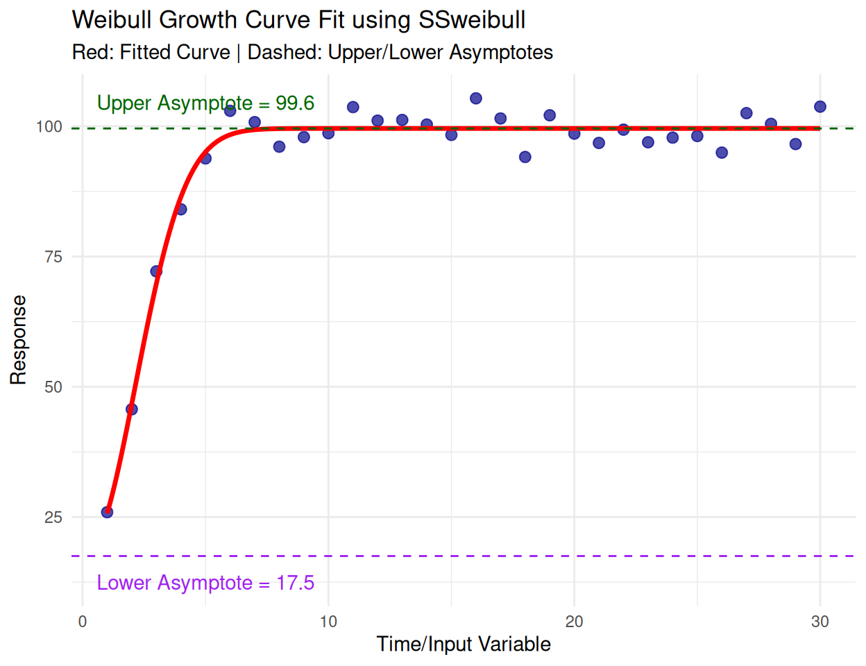

Gompertz Growth Model: `SSgompertz`

Model:

$y = Asym \cdot e^{-b_2 \cdot e^{-b_3 \cdot x}}$
Parameters:
- Asym: Asymptote.
- b2: Displacement along the x-axis.
- b3: Growth rate.

Code

# Create example data
set.seed(123)
x <- 1:10
y <- 100 * exp(-exp(2 - 0.3 * x)) + rnorm(10, sd = 5)
data <- data.frame(x = x, y = y)

# Fit the Gompertz Growth Model using SSgompertz
fit <- nls(y ~ SSgompertz(x, Asym, b2, b3), data = data)
summary(fit)


Formula: y ~ SSgompertz(x, Asym, b2, b3)

Parameters:
     Estimate Std. Error t value Pr(>|t|)    
Asym 87.88811   20.69380   4.247  0.00381 ** 
b2    6.00060    1.85009   3.243  0.01419 *  
b3    0.74290    0.06791  10.939 1.18e-05 ***
---
Signif. codes:  0 '***' 0.001 '**' 0.01 '*' 0.05 '.' 0.1 ' ' 1

Residual standard error: 4.416 on 7 degrees of freedom

Number of iterations to convergence: 0 
Achieved convergence tolerance: 1.909e-06

Code

# Extract fitted values
data$fitted <- predict(fit)

# Plot the data and the fitted model using ggplot2
ggplot(data, aes(x = x, y = y)) +
  geom_point(color = 'blue', size = 2) +
  geom_line(aes(y = fitted), color = 'red', size = 1) +
  labs(title = "Gompertz Growth Model",
       x = "X",
       y = "Y") +
  theme_minimal()

Warning: Using `size` aesthetic for lines was deprecated in ggplot2 3.4.0.
ℹ Please use `linewidth` instead.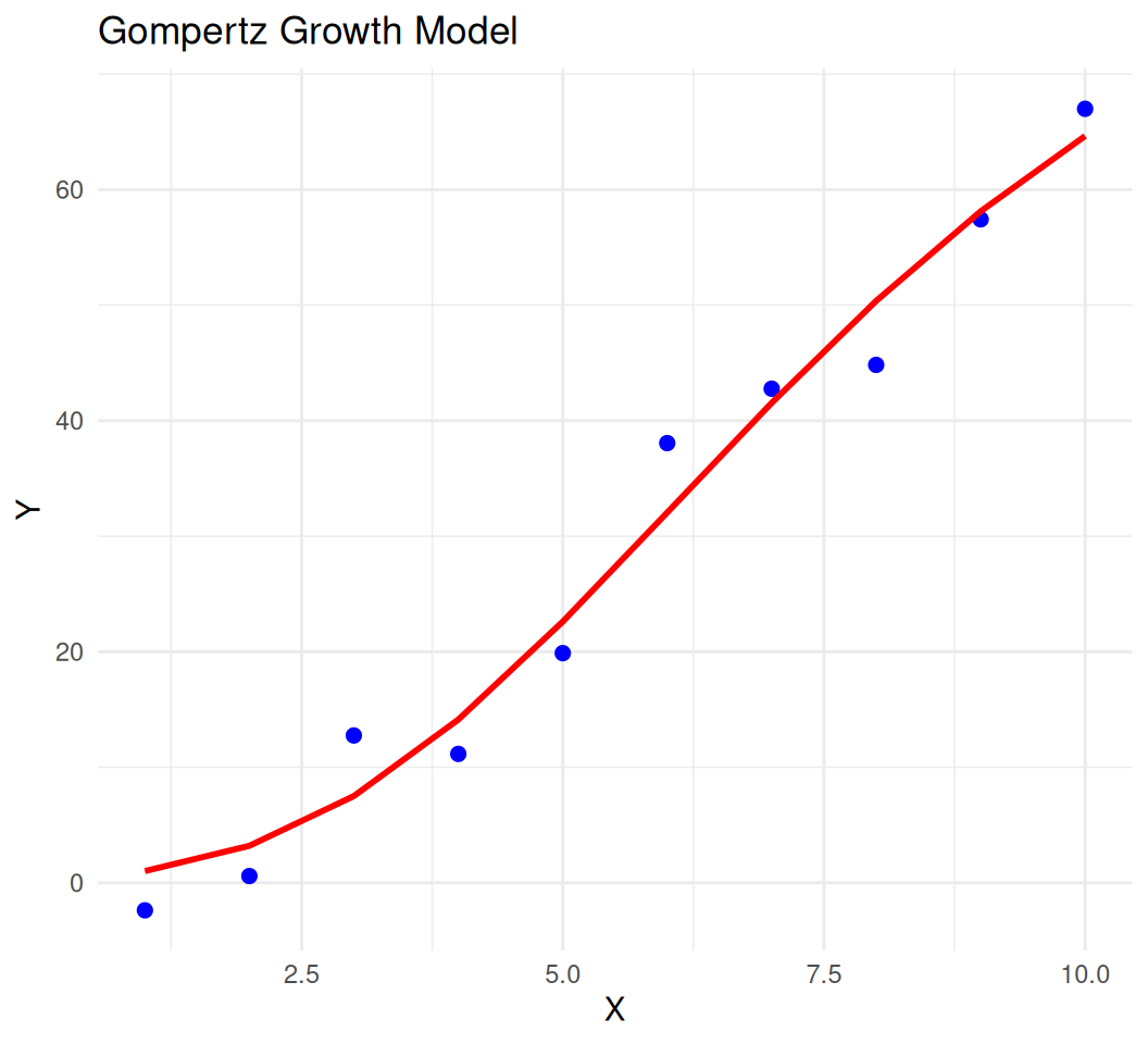

Asymptotic Regression: `SSasymp`

Model:

$y = Asym + (R_0 - Asym) e^{-e^{lrc} \cdot x}$
Parameters:
- Asym: Horizontal asymptote.
- R0: y-intercept (at (x = 0)).

Code

set.seed(123)
   x <- 1:30
   y <- SSasymp(x, Asym = 50, R0 = 100, lrc = log(0.1)) + rnorm(30, sd = 2)
   df <- data.frame(x, y)
   
   fit <- nls(y ~ SSasymp(x, Asym, R0, lrc), data = df)
   summary(fit)


Formula: y ~ SSasymp(x, Asym, R0, lrc)

Parameters:
     Estimate Std. Error t value Pr(>|t|)    
Asym  48.4343     1.5058   32.16   <2e-16 ***
R0   100.0796     1.6400   61.02   <2e-16 ***
lrc   -2.3718     0.0936  -25.34   <2e-16 ***
---
Signif. codes:  0 '***' 0.001 '**' 0.01 '*' 0.05 '.' 0.1 ' ' 1

Residual standard error: 1.97 on 27 degrees of freedom

Number of iterations to convergence: 0 
Achieved convergence tolerance: 2.202e-07

Code

   # Plot
   ggplot(df, aes(x, y)) +
     geom_point() +
     geom_smooth(method = "nls", formula = y ~ SSasymp(x, Asym, R0, lrc),
                 se = FALSE, color = "blue") +
     ggtitle("Asymptotic Regression with SSasymp")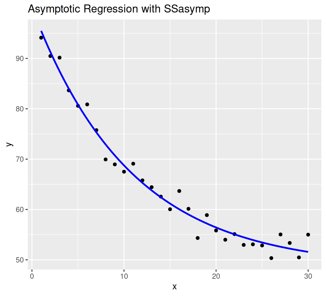

Michaelis-Menten Model: `SSmicmen`

Model:

$y = \frac{V_m \cdot x}{K + x}$)

Parameters:
- Vm: Maximum reaction rate.
- K: Substrate concentration at half of $V_m$.

Code

set.seed(123)
x <- seq(0, 50, by = 5)
y <- SSmicmen(x, Vm = 10, K = 5) + rnorm(length(x), sd = 0.5)
df <- data.frame(x, y)
   
# Get reasonable starting values
Vm_start <- max(df$y) * 1.1  # Slightly above observed max
K_start <- median(df$x[df$y >= 0.5 * max(df$y)])  # x near half-maximal response

# Fit model
fit <- nls(
  y ~ SSmicmen(x, Vm, K),
  data = df,
  start = list(Vm = Vm_start, K = K_start),
  control = nls.control(warnOnly = TRUE)  # Show warnings instead of errors
)

# Check results
summary(fit)


Formula: y ~ SSmicmen(x, Vm, K)

Parameters:
   Estimate Std. Error t value Pr(>|t|)    
Vm   9.9403     0.3781  26.293 8.04e-10 ***
K    4.4053     0.9343   4.715   0.0011 ** 
---
Signif. codes:  0 '***' 0.001 '**' 0.01 '*' 0.05 '.' 0.1 ' ' 1

Residual standard error: 0.4946 on 9 degrees of freedom

Number of iterations to convergence: 6 
Achieved convergence tolerance: 4.157e-06

Code

# Plot
ggplot(df, aes(x, y)) +
     geom_point() +
     stat_function(fun = function(x) coef(fit)[1] * x / (coef(fit)[2] + x),
                   color = "green") +
     ggtitle("Michaelis-Menten Fit with SSmicmen")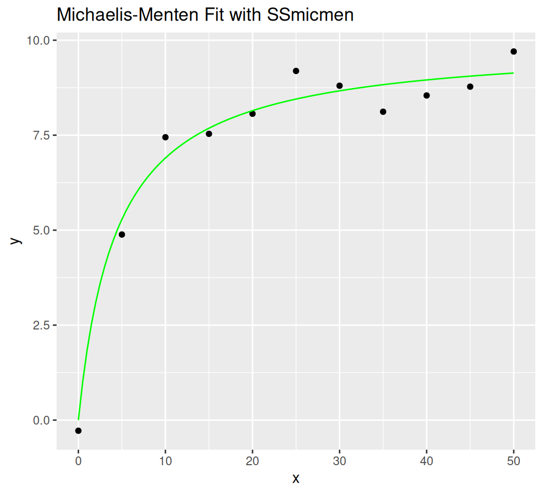

Summary and Conclusion

This tutorial explored the concept of self-starting functions in R, which are useful for fitting non-linear models. Self-starting functions provide initial parameter estimates that help the fitting algorithm converge more efficiently. We discussed several key self-starting functions, including the logistic model, four-parameter logistic model, Weibull growth curve, Gompertz growth model, asymptotic regression, and Michaelis-Menten model. For each function, we provided a brief description, example code, and visualization to demonstrate how to use them in practice. By leveraging self-starting functions, you can streamline the process of fitting non-linear models and obtain more reliable results.

References

The-R Book by Michael J. Crawley
A collection of self-starters for nonlinear regression in R - This article on R-bloggers discusses various self-starting functions available in R and how they can be used to simplify non-linear regression analysis.
Self-starting routines for nonlinear regression models - Another article on R-bloggers that delves into self-starting routines provided by the drc package, useful for dose-response analyses and other biological processes.
Some useful equations for nonlinear regression in R - This resource on StatForBiology provides useful equations and discusses the convenience of using self-starting routines in non-linear regression models.
Self-starting routines for nonlinear regression models - This article on StatForBiology explains the benefits of using self-starting functions in R for fitting non-linear models, especially in biological research.

6. Self-starting Function

Important Self-starting Functions

Install Required R Packages

Load R Packages

Logistic Growth Model: SSlogis

Four-Parameter Logistic Model: SSfpl

Weibull Growth Curve: SSweibull

Gompertz Growth Model: SSgompertz

Asymptotic Regression: SSasymp

Michaelis-Menten Model: SSmicmen

Summary and Conclusion

References

Logistic Growth Model: `SSlogis`

Four-Parameter Logistic Model: `SSfpl`

Weibull Growth Curve: `SSweibull`

Gompertz Growth Model: `SSgompertz`

Asymptotic Regression: `SSasymp`

Michaelis-Menten Model: `SSmicmen`