8. Beta Regression

Beta regression is a statistical modeling technique for continuous response variables within the interval ($0, 1$). This makes it particularly suitable for data such as proportions, rates, and probabilities, like conversion rates in marketing campaigns or percentage allocations. In this tutorial, we will demonstrate the entire process using synthetic data. We’ll cover data generation, model fitting, and performance metrics, including pseudo $R^2$ and model coefficients, all without relying on any built-in R packages. Following this, we will simplify the modeling of beta regression by utilizing the betareg() function from the {betareg} package and demonstrate how to interpret the results practically. Additionally, we will explore the marginal effects and assess the model’s performance through cross-validation. This hands-on introduction will equip you with the necessary skills to apply beta regression to real-world datasets with bounded response variables.

Overview

Beta regression is a type of regression model used when the dependent variable $y$ is continuous and constrained within an interval, typically $(0, 1)$. This is common for proportions or rates, like percentages (excluding 0 and 1). Traditional linear regression models don’t work well in these cases, as they can predict values outside the $(0, 1)$ interval, and assumptions of normality and homoscedasticity may not hold. Beta regression is built on the beta distribution, which is well-suited for modeling such bounded data.

Here’s a step-by-step explanation of beta regression, including key mathematical details.

Understanding the Beta Distribution

The beta distribution is a continuous probability distribution defined on the interval $(0, 1)$. Its probability density function is given by:

\[ f(y; \alpha, \beta) = \frac{y^{\alpha - 1} (1 - y)^{\beta - 1}}{B(\alpha, \beta)} \]

where:

$ y (0, 1) $ is the variable of interest.
$> 0 $ and $\beta > 0$ are shape parameters.
$B(\alpha, \beta)$ is the beta function, which normalizes the distribution:

\[ B(\alpha, \beta) = \int_0^1 t^{\alpha - 1} (1 - t)^{\beta - 1} \, dt \]

The mean $\mu$ and variance $\sigma^2$ of a beta distribution are given by:

\[ \mu = \frac{\alpha}{\alpha + \beta}, \quad \sigma^2 = \frac{\alpha \beta}{(\alpha + \beta)^2 (\alpha + \beta + 1)} \]

The mean $\mu$ represents the central tendency, while the variance $\sigma^2$ reflects the spread.

Modeling the Mean with a Link Function

In beta regression, we model the mean $\mu$ of the beta distribution as a function of the predictors $X$. Since $\mu \in (0, 1)$), we apply a link function $g(\cdot)$ to transform $\mu$ into an unbounded linear predictor:

\[ g(\mu) = X \beta \]

Common choices for the link function $g(\cdot)$ are:

The logit link: $g(\mu) = \log \left( \frac{\mu}{1 - \mu} \right)$
The probit link: $g(\mu) = \Phi^{-1}(\mu)$, where $\Phi^{-1}$ is the inverse CDF of the normal distribution

The link function ensures that $\mu$ lies between 0 and 1, regardless of the values of $X$.

Specifying the Dispersion Parameter

In addition to the mean, beta regression also incorporates a precision (or dispersion) parameter, often denoted by $\phi$. The parameters $\alpha$ and $\beta$ can be reparametrized in terms of $\mu$ and $\phi$ as follows:

\[ \alpha = \mu \phi, \quad \beta = (1 - \mu) \phi \]

Here, $\phi$ is related to the variance of $y$), with larger values of $\phi$ leading to a smaller variance. Unlike in ordinary regression, where variance is typically constant, in beta regression, the dispersion parameter $\phi$ allows for flexibility in the variability of $y$ based on the values of the predictors.

Defining the Likelihood Function

The likelihood function for beta regression is based on the beta distribution’s PDF. Given ( n ) observations, the likelihood function is:

\[ L(\beta, \phi; y) = \prod_{i=1}^n f(y_i; \mu_i, \phi) = \prod_{i=1}^n \frac{y_i^{\mu_i \phi - 1} (1 - y_i)^{(1 - \mu_i) \phi - 1}}{B(\mu_i \phi, (1 - \mu_i) \phi)} \]

Taking the logarithm of the likelihood function (for simplicity in optimization) gives the log-likelihood:

\[ \log L(\beta, \phi; y) = \sum_{i=1}^n \left[ (\mu_i \phi - 1) \log y_i + ((1 - \mu_i) \phi - 1) \log (1 - y_i) - \log B(\mu_i \phi, (1 - \mu_i) \phi) \right] \]

Estimating Parameters Using Maximum Likelihood

To estimate the parameters $\beta$ and $\phi$, we maximize the log-likelihood function. This is often done using numerical optimization techniques because the log-likelihood function is complex and does not have a closed-form solution.

The parameter estimates $\hat{\beta}$ and $\hat{\phi}$ are obtained by solving:

\[ \frac{\partial \log L}{\partial \beta} = 0 \quad \text{and} \quad \frac{\partial \log L}{\partial \phi} = 0 \]

Once these parameters are estimated, they can be used to predict the mean response $\mu$ for new data points.

Interpreting the Model

After fitting a beta regression model, we interpret $\beta$ coefficients in terms of their effect on the log-odds (if using the logit link) of the mean $\mu$. A positive $\beta_j$ implies that an increase in $X_j$ is associated with an increase in the mean of $y$, while a negative $\beta_j$ implies the opposite.

The dispersion parameter ( ) provides insight into the variability of ( y ): a high ( ) implies that the values of ( y ) are tightly clustered around the mean, while a low ( ) suggests more variability.

Beta Regression Model from Scratch

To demonstrate beta regression in R without using any specialized package, we’ll need to work directly with the beta distribution and likelihood functions. This example will walk through generating synthetic data, defining the likelihood function for beta regression, estimating parameters with numerical optimization, and evaluating model performance.

Generate Synthetic Data

We’ll generate synthetic data with four predictors and a target variable $y$) constrained between $(0, 1)$ We’ll simulate the beta-distributed response $y$ based on a linear combination of the predictors transformed through a logistic function to ensure values stay in the $(0, 1)$ range.

Code

# set seeds for reproducibility
set.seed(123)

# Generate predictors
n <- 100
X1 <- rnorm(n, mean = 0, sd = 1)
X2 <- rnorm(n, mean = 0, sd = 1)
X3 <- rnorm(n, mean = 0, sd = 1)
X4 <- rnorm(n, mean = 0, sd = 1)

# Define true coefficients
beta <- c(0.5, -0.3, 0.8, -0.2, 0.1) # Intercept + 4 predictors
phi <- 10 # Dispersion parameter

# Calculate the linear predictor and apply logistic link function to get mu
linear_predictor <- beta[1] + beta[2]*X1 + beta[3]*X2 + beta[4]*X3 + beta[5]*X4
mu <- 1 / (1 + exp(-linear_predictor))

# Generate beta-distributed response variable y
alpha <- mu * phi
beta_param <- (1 - mu) * phi
y <- rbeta(n, alpha, beta_param)

# Combine data into a data frame
data <- data.frame(y = y, X1 = X1, X2 = X2, X3 = X3, X4 = X4)
head(data)

          y          X1          X2         X3         X4
1 0.3857103 -0.56047565 -0.71040656  2.1988103 -0.7152422
2 0.7940054 -0.23017749  0.25688371  1.3124130 -0.7526890
3 0.3384641  1.55870831 -0.24669188 -0.2651451 -0.9385387
4 0.4915856  0.07050839 -0.34754260  0.5431941 -1.0525133
5 0.5579215  0.12928774 -0.95161857 -0.4143399 -0.4371595
6 0.8024065  1.71506499 -0.04502772 -0.4762469  0.3311792

Define the Beta Regression Log-Likelihood Function

We’ll create a function to compute the log-likelihood of the beta regression model. The function takes the model parameters (coefficients $\beta$ and dispersion parameter $\phi$) and the data as input and returns the negative log-likelihood. We use the dbeta() function from the stats package to calculate the log-likelihood for each observation.

Code

log_likelihood <- function(params, data) {
  # Extract parameters
  beta <- params[1:5]      # coefficients (intercept + 4 predictors)
  phi <- exp(params[6])     # dispersion parameter, transformed to be positive

  # Linear predictor
  X <- as.matrix(cbind(1, data[, -1])) # Add intercept to predictors matrix
  linear_predictor <- X %*% beta
  mu <- 1 / (1 + exp(-linear_predictor)) # Logistic link function
  
  # Calculate alpha and beta parameters of the beta distribution
  alpha <- mu * phi
  beta_param <- (1 - mu) * phi

  # Log-likelihood calculation
  ll <- sum(dbeta(data$y, alpha, beta_param, log = TRUE))
  return(-ll) # Return negative log-likelihood for minimization
}

Fit the Model Using Numerical Optimization

We’ll use optim() to minimize the negative log-likelihood and estimate the parameters. We start with random initial guesses for the parameters and use the BFGS optimization method. The hessian = TRUE argument allows us to approximate standard errors later.

Code

# Initial parameter guesses (random starting values)
initial_params <- c(0, 0, 0, 0, 0, log(1))

# Optimize
fit <- optim(par = initial_params, fn = log_likelihood, data = data, method = "BFGS", hessian = TRUE)

# Extract estimated parameters
beta_hat <- fit$par[1:5]
phi_hat <- exp(fit$par[6])

cat("Estimated coefficients (beta):\n", beta_hat, "\n")

Estimated coefficients (beta):
 0.5446189 -0.1674559 0.8265935 -0.3049972 0.06331931

Code

cat("Estimated dispersion parameter (phi):\n", phi_hat, "\n")

Estimated dispersion parameter (phi):
 9.908912

Display Model Summary

Let’s create a summary table for the estimated coefficients and their standard errors. The hessian matrix from optim() can be used to approximate standard errors.

Code

# Standard errors from the Hessian
se <- sqrt(diag(solve(fit$hessian)))
# Extract estimated coefficients and phi
beta_est <- fit$par[1:5]
phi_est <- exp(fit$par[6])  # Inverse of log transformation

# Print results
summary_table <- data.frame(Coefficient = c("Intercept", "X1", "X2", "X3", "X4"),
                            Estimate = beta_est)
summary_table

  Coefficient    Estimate
1   Intercept  0.54461892
2          X1 -0.16745590
3          X2  0.82659346
4          X3 -0.30499722
5          X4  0.06331931

Dispersion Parameter

Code

# Dispersion parameter has already been calculated as phi_est
cat("Dispersion Parameter (phi) from the model:", phi_est, "\n")

Dispersion Parameter (phi) from the model: 9.908912

Evaluate Model Performance

We’ll use the estimated parameters to compute the fitted values of ( $\mu$ ) and check the model’s performance by comparing predicted values to actual values.

Code

# Compute predicted values of mu
linear_predictor_hat <- as.matrix(cbind(1, data[, -1])) %*% beta_hat
mu_hat <- 1 / (1 + exp(-linear_predictor_hat))

# Mean Squared Error (MSE) as a performance metric
mse <- mean((data$y - mu_hat)^2)
cat("Mean Squared Error (MSE):\n", mse, "\n")

Mean Squared Error (MSE):
 0.01861497

Cross-validation

To evaluate the beta regression model using cross-validation, we can use a simple $k$-fold cross-validation approach. Cross-validation will split the data into k subsets, train the model on $k−1$ folds, and evaluate it on the remaining fold. We repeat this process $k$ times, each time using a different fold for validation.

Here’s how to implement $k$-fold cross-validation for the beta regression model created earlier. We’ll compute the Mean Squared Error (MSE) for each fold as a performance metric and calculate the average MSE across all folds.

Code

# Step 1: Define Cross-Validation Function
cross_validate_beta_regression <- function(data, k = 5) {
  n <- nrow(data)
  indices <- sample(1:n)  # Shuffle data
  fold_size <- floor(n / k)
  
  mse_values <- numeric(k)  # To store MSE for each fold
  
  for (i in 1:k) {
    # Define training and validation indices
    val_indices <- indices[((i - 1) * fold_size + 1):(i * fold_size)]
    train_data <- data[-val_indices, ]
    val_data <- data[val_indices, ]
    
    # Fit the model on training data
    initial_params <- c(0, 0, 0, 0, 0, log(1))
    fit <- optim(par = initial_params, fn = log_likelihood, data = train_data, method = "BFGS")
    
    # Extract the estimated parameters
    beta_hat <- fit$par[1:5]
    phi_hat <- exp(fit$par[6])
    
    # Compute predictions for validation data
    X_val <- as.matrix(cbind(1, val_data[, -1]))  # Add intercept
    linear_predictor_val <- X_val %*% beta_hat
    mu_val <- 1 / (1 + exp(-linear_predictor_val))  # Predicted mean for validation data
    
    # Calculate MSE for this fold
    mse_values[i] <- mean((val_data$y - mu_val)^2)
  }
  
  # Return average MSE across all folds
  avg_mse <- mean(mse_values)
  return(avg_mse)
}

# Step 2: Run Cross-Validation
set.seed(123)
k <- 5
avg_mse_cv <- cross_validate_beta_regression(data, k)
cat("Average Cross-Validated MSE:", avg_mse_cv, "\n")

Average Cross-Validated MSE: 0.02046396

Beta Regression in R

In beta regression, we model the mean of the response variable (proportion) through a link function (usually a logit or log-log link) to keep predictions within the 0-1 range. The mean prediction of the response variable is often interpreted as the central tendency of the outcome for given levels of the predictors.

Install Required R Packages

Following R packages are required to run this notebook. If any of these packages are not installed, you can install them using the code below:

Code

packages <- c('tidyverse',
     'plyr',
      'DataExplorer',
         'dlookr',
         'rstatix',
       'flextable',
         'gtsummary',
         'performance',
       'report',
         'sjPlot',
         'margins',
         'marginaleffects',
         'ggeffects',
         'patchwork',
         'metrica',
         'MASS',
     'betareg',
    'lmtest'
        )

#| warning: false
#| error: false

# Install missing packages
new_packages <- packages[!(packages %in% installed.packages()[,"Package"])]
if(length(new_packages)) install.packages(new_packages)

# Verify installation
cat("Installed packages:\n")
print(sapply(packages, requireNamespace, quietly = TRUE))

Load R-packages

Code

# Load packages with suppressed messages
invisible(lapply(packages, function(pkg) {
  suppressPackageStartupMessages(library(pkg, character.only = TRUE))
}))

Code

# Check loaded packages
cat("Successfully loaded packages:\n")

Successfully loaded packages:

Code

print(search()[grepl("package:", search())])

 [1] "package:lmtest"          "package:zoo"            
 [3] "package:betareg"         "package:MASS"           
 [5] "package:metrica"         "package:patchwork"      
 [7] "package:ggeffects"       "package:marginaleffects"
 [9] "package:margins"         "package:sjPlot"         
[11] "package:report"          "package:performance"    
[13] "package:gtsummary"       "package:flextable"      
[15] "package:rstatix"         "package:dlookr"         
[17] "package:DataExplorer"    "package:plyr"           
[19] "package:lubridate"       "package:forcats"        
[21] "package:stringr"         "package:dplyr"          
[23] "package:purrr"           "package:readr"          
[25] "package:tidyr"           "package:tibble"         
[27] "package:ggplot2"         "package:tidyverse"      
[29] "package:stats"           "package:graphics"       
[31] "package:grDevices"       "package:utils"          
[33] "package:datasets"        "package:methods"        
[35] "package:base"

Data

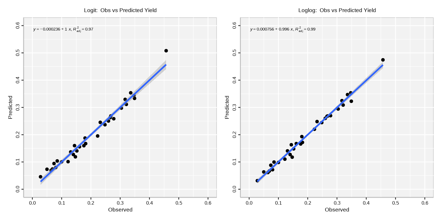
In this tutorial, we will use Prater’s well-known gasoline yield data from 1956. The primary variable of interest is yield, which represents the proportion of crude oil converted to gasoline after distillation and fractionation. A beta regression model is particularly suitable for analyzing this variable. We also have two explanatory variables: temp, the temperature (measured in degrees Fahrenheit) at which all the gasoline has vaporized, and batch, a categorical variable denoting ten unique batches of conditions involved in the experiments based on various other factors.

Source: Prater NH (1956). “Estimate Gasoline Yields from Crudes.” Petroleum Refiner, 35(5), 236–238.

Code

data("GasolineYield", package = "betareg") 
glimpse(GasolineYield)

Rows: 32
Columns: 6
$ yield    <dbl> 0.122, 0.223, 0.347, 0.457, 0.080, 0.131, 0.266, 0.074, 0.182…
$ gravity  <dbl> 50.8, 50.8, 50.8, 50.8, 40.8, 40.8, 40.8, 40.0, 40.0, 40.0, 3…
$ pressure <dbl> 8.6, 8.6, 8.6, 8.6, 3.5, 3.5, 3.5, 6.1, 6.1, 6.1, 6.1, 6.1, 6…
$ temp10   <dbl> 190, 190, 190, 190, 210, 210, 210, 217, 217, 217, 220, 220, 2…
$ temp     <dbl> 205, 275, 345, 407, 218, 273, 347, 212, 272, 340, 235, 300, 3…
$ batch    <fct> 1, 1, 1, 1, 2, 2, 2, 3, 3, 3, 4, 4, 4, 4, 5, 5, 5, 6, 6, 6, 7…

First we use We use diagnose() function of {dlookr} package to do general general diagnosis of all variables.

Code

#library (flextable)
dlookr::diagnose(GasolineYield) |>  
  flextable()

variables	types	unique_count	unique_rate
yield	numeric	32	1.00000
gravity	numeric	9	0.28125
pressure	numeric	9	0.28125
temp10	numeric	10	0.31250
temp	numeric	28	0.87500
batch	factor	10	0.31250

Fit Beta Models in R

betareg() function fit beta regression models for rates and proportions via maximum likelihood using a parametrization with mean (depending through a link function on the covariates) and precision parameter (called phi). The argument of betareg(0) are:

betareg(formula, data, subset, na.action, weights, offset,
  link = c("logit", "probit", "cloglog", "cauchit", "log", "loglog"),
  link.phi = NULL, type = c("ML", "BC", "BR"), dist = NULL, nu = NULL,
  control = betareg.control(...), model = TRUE,
  y = TRUE, x = FALSE, ...)

The link for the $\Phi_{i}$ precision equation can be changed by link.phi in both cases where identity, log, and sqrt are allowed as admissible values. The default for the $\mu$ mean equation is always the logit link but all link functions for the binomial family in glm() are allowed as well as the log-log link: “logit, probit, cloglog, cauchit, `log, and”loglog”.

Standard Beta Regression Model

First, we will fit betareg model where yield depends on batch and temp, using the standard logit link function:

Code

# Standard Beta Regression Model
fit.beta.01<-betareg(yield ~ batch + temp, data = GasolineYield)
summary(fit.beta.01)


Call:
betareg(formula = yield ~ batch + temp, data = GasolineYield)

Quantile residuals:
    Min      1Q  Median      3Q     Max 
-2.1396 -0.5698  0.1202  0.7040  1.7506 

Coefficients (mean model with logit link):
              Estimate Std. Error z value Pr(>|z|)    
(Intercept) -6.1595710  0.1823247 -33.784  < 2e-16 ***
batch1       1.7277289  0.1012294  17.067  < 2e-16 ***
batch2       1.3225969  0.1179020  11.218  < 2e-16 ***
batch3       1.5723099  0.1161045  13.542  < 2e-16 ***
batch4       1.0597141  0.1023598  10.353  < 2e-16 ***
batch5       1.1337518  0.1035232  10.952  < 2e-16 ***
batch6       1.0401618  0.1060365   9.809  < 2e-16 ***
batch7       0.5436922  0.1091275   4.982 6.29e-07 ***
batch8       0.4959007  0.1089257   4.553 5.30e-06 ***
batch9       0.3857930  0.1185933   3.253  0.00114 ** 
temp         0.0109669  0.0004126  26.577  < 2e-16 ***

Phi coefficients (precision model with identity link):
      Estimate Std. Error z value Pr(>|z|)    
(phi)    440.3      110.0   4.002 6.29e-05 ***
---
Signif. codes:  0 '***' 0.001 '**' 0.01 '*' 0.05 '.' 0.1 ' ' 1 

Type of estimator: ML (maximum likelihood)
Log-likelihood:  84.8 on 12 Df
Pseudo R-squared: 0.9617
Number of iterations: 51 (BFGS) + 3 (Fisher scoring)

Batch and temperature are both significant predictors of yield in the GasolineYield data.
Higher values of batch and temp are associated with an increase in the mean gasoline yield, meaning these factors positively influence yield when considered individually.

The high value of the dispersion parameter ($\Phi$) (492.0) suggests that gasoline yields in the data are relatively consistent around their predicted means for the given conditions, which may indicate a good fit (less dispersion).

Variable Dispersion Beta Regression Model

In standard beta regression, the dispersion parameter $\Phi$ controls the variability of the response variable around its mean. A single (constant) $\Phi$ is estimated for the entire model, implying that all observations have the same degree of variability around the mean.

In a variable dispersion model, we allow the dispersion parameter $\Phi$ to vary based on one or more predictor variables. This means that $\Phi$ itself is modeled as a function of some variables, just like the mean. Variable dispersion models are useful when:

The variability of the response is expected to differ across certain levels of predictors. For example, in a clinical trial, patients from different treatment groups may exhibit varying response variability.
The residuals from a standard beta regression model show patterns that suggest unequal dispersion across values of certain predictors.

Code

# Variable Dispersion Beta Regression Model  
fit.beta.02<-betareg(yield ~ batch + temp | temp, data = GasolineYield)
summary(fit.beta.02)


Call:
betareg(formula = yield ~ batch + temp | temp, data = GasolineYield)

Quantile residuals:
    Min      1Q  Median      3Q     Max 
-2.1040 -0.5852 -0.1425  0.6899  2.5203 

Coefficients (mean model with logit link):
              Estimate Std. Error z value Pr(>|z|)    
(Intercept) -5.9232361  0.1835262 -32.275  < 2e-16 ***
batch1       1.6019877  0.0638561  25.087  < 2e-16 ***
batch2       1.2972663  0.0991001  13.090  < 2e-16 ***
batch3       1.5653383  0.0997392  15.694  < 2e-16 ***
batch4       1.0300720  0.0632882  16.276  < 2e-16 ***
batch5       1.1541630  0.0656427  17.582  < 2e-16 ***
batch6       1.0194446  0.0663510  15.364  < 2e-16 ***
batch7       0.6222591  0.0656325   9.481  < 2e-16 ***
batch8       0.5645830  0.0601846   9.381  < 2e-16 ***
batch9       0.3594390  0.0671406   5.354 8.63e-08 ***
temp         0.0103595  0.0004362  23.751  < 2e-16 ***

Phi coefficients (precision model with log link):
            Estimate Std. Error z value Pr(>|z|)    
(Intercept) 1.364089   1.225781   1.113    0.266    
temp        0.014570   0.003618   4.027 5.65e-05 ***
---
Signif. codes:  0 '***' 0.001 '**' 0.01 '*' 0.05 '.' 0.1 ' ' 1 

Type of estimator: ML (maximum likelihood)
Log-likelihood: 86.98 on 13 Df
Pseudo R-squared: 0.9519
Number of iterations: 33 (BFGS) + 28 (Fisher scoring)

The Beta Regression with `loh-log` link function

In binomial Generalized Linear Models (GLMs), choosing the right link function is crucial for enhancing model fit, particularly when the data includes extreme proportions (values close to 0 or 1). In such cases, we will use log-log link function instead of the default logit link.

Code

# Beta Regression Model  with loglog link function
fit.beta.03<-betareg(yield ~ batch + temp , 
                      data = GasolineYield,
                      link = "loglog")
summary(fit.beta.03)


Call:
betareg(formula = yield ~ batch + temp, data = GasolineYield, link = "loglog")

Quantile residuals:
    Min      1Q  Median      3Q     Max 
-1.7440 -0.7260  0.1112  0.6855  2.5924 

Coefficients (mean model with loglog link):
              Estimate Std. Error z value Pr(>|z|)    
(Intercept) -2.7937944  0.0579177 -48.237  < 2e-16 ***
batch1       0.9038714  0.0347387  26.019  < 2e-16 ***
batch2       0.6553991  0.0376683  17.399  < 2e-16 ***
batch3       0.7684237  0.0378459  20.304  < 2e-16 ***
batch4       0.5375955  0.0335027  16.046  < 2e-16 ***
batch5       0.5516613  0.0346755  15.909  < 2e-16 ***
batch6       0.5198331  0.0351349  14.795  < 2e-16 ***
batch7       0.2921514  0.0340681   8.576  < 2e-16 ***
batch8       0.2504792  0.0349788   7.161 8.02e-13 ***
batch9       0.1871284  0.0383089   4.885 1.04e-06 ***
temp         0.0053645  0.0001341  40.008  < 2e-16 ***

Phi coefficients (precision model with identity link):
      Estimate Std. Error z value Pr(>|z|)    
(phi)    906.7      226.6   4.001 6.32e-05 ***
---
Signif. codes:  0 '***' 0.001 '**' 0.01 '*' 0.05 '.' 0.1 ' ' 1 

Type of estimator: ML (maximum likelihood)
Log-likelihood: 96.16 on 12 Df
Pseudo R-squared: 0.9852
Number of iterations: 51 (BFGS) + 2 (Fisher scoring)

Variable dispersion shows a significant improvement with the inclusion of the temp regressor.

The Beta Regression with `link.phi = "log"` link function

Typically, a log-link leads to somewhat improved quadratic approximations of the likelihood and less iterations in the optimization. For example, refitting fit.beat.03 (loglog model) with g2(·) = log(·) converges more quickly:

Code

# Beta Regression Model  with loglog link function
fit.beta.04<- update(fit.beta.03, link.phi = "log")
summary(fit.beta.04)


Call:
betareg(formula = yield ~ batch + temp, data = GasolineYield, link = "loglog", 
    link.phi = "log")

Quantile residuals:
    Min      1Q  Median      3Q     Max 
-1.7440 -0.7260  0.1112  0.6855  2.5924 

Coefficients (mean model with loglog link):
              Estimate Std. Error z value Pr(>|z|)    
(Intercept) -2.7937944  0.0579177 -48.237  < 2e-16 ***
batch1       0.9038714  0.0347387  26.019  < 2e-16 ***
batch2       0.6553991  0.0376683  17.399  < 2e-16 ***
batch3       0.7684237  0.0378459  20.304  < 2e-16 ***
batch4       0.5375955  0.0335027  16.046  < 2e-16 ***
batch5       0.5516613  0.0346755  15.909  < 2e-16 ***
batch6       0.5198331  0.0351349  14.795  < 2e-16 ***
batch7       0.2921514  0.0340681   8.576  < 2e-16 ***
batch8       0.2504792  0.0349788   7.161 8.02e-13 ***
batch9       0.1871284  0.0383089   4.885 1.04e-06 ***
temp         0.0053645  0.0001341  40.008  < 2e-16 ***

Phi coefficients (precision model with log link):
            Estimate Std. Error z value Pr(>|z|)    
(Intercept)     6.81       0.25   27.24   <2e-16 ***
---
Signif. codes:  0 '***' 0.001 '**' 0.01 '*' 0.05 '.' 0.1 ' ' 1 

Type of estimator: ML (maximum likelihood)
Log-likelihood: 96.16 on 12 Df
Pseudo R-squared: 0.9852
Number of iterations: 21 (BFGS) + 2 (Fisher scoring)

with a lower number of iterations than for gy_loglog which had 51 iterations.

Model Comparison

We will use lrtest{} of {lmtest} package for comparisons of models via asymptotic likelihood ratio tests.

Code

library(lmtest)
lrtest(fit.beta.01, fit.beta.02,fit.beta.03)

Likelihood ratio test

Model 1: yield ~ batch + temp
Model 2: yield ~ batch + temp | temp
Model 3: yield ~ batch + temp
  #Df LogLik Df  Chisq Pr(>Chisq)    
1  12 84.798                         
2  13 86.977  1  4.359    0.03681 *  
3  12 96.155 -1 18.356  1.832e-05 ***
---
Signif. codes:  0 '***' 0.001 '**' 0.01 '*' 0.05 '.' 0.1 ' ' 1

Code

AIC(fit.beta.01, fit.beta.02,fit.beta.03)

            df       AIC
fit.beta.01 12 -145.5951
fit.beta.02 13 -147.9541
fit.beta.03 12 -168.3101

The temp were included as a regressor in the precision equation of logit.03, it would no longer yield significant improvements. Thus, improvement of the model fit in the mean equation by adoption of the log-log link have waived the need for a variable precision equation.

Code

lrtest(fit.beta.01, . ~ . + I(predict(fit.beta.01, type = "link")^2))

Likelihood ratio test

Model 1: yield ~ batch + temp
Model 2: yield ~ batch + temp + I(predict(fit.beta.01, type = "link")^2)
  #Df LogLik Df  Chisq Pr(>Chisq)    
1  12 84.798                         
2  13 96.001  1 22.407  2.205e-06 ***
---
Signif. codes:  0 '***' 0.001 '**' 0.01 '*' 0.05 '.' 0.1 ' ' 1

Code

lrtest(fit.beta.03, . ~ . + I(predict(fit.beta.03, type = "link")^2))

Likelihood ratio test

Model 1: yield ~ batch + temp
Model 2: yield ~ batch + temp + I(predict(fit.beta.03, type = "link")^2)
  #Df LogLik Df  Chisq Pr(>Chisq)
1  12 96.155                     
2  13 96.989  1 1.6671     0.1966

The improvement of the model fit can also be brought out graphically in a display of predicted vs. observed values”

Code

logit.df<-cbind.data.frame(Obs = GasolineYield$yield, Pred = fit.beta.01$fitted.values ) 
loglog.df<-cbind.data.frame(Obs = GasolineYield$yield, Pred = fit.beta.03$fitted.values )

Code

library(ggpmisc)

Loading required package: ggpp

Registered S3 methods overwritten by 'ggpp':
  method                  from   
  heightDetails.titleGrob ggplot2
  widthDetails.titleGrob  ggplot2


Attaching package: 'ggpp'

The following object is masked from 'package:ggplot2':

    annotate

Code

formula<-y~x

p1<-ggplot(logit.df, aes(Obs,Pred)) +
  geom_point() +
    geom_smooth(method = "lm")+
  stat_poly_eq(use_label(c("eq", "adj.R2")), formula = formula) +
  ggtitle("Logit:  Obs vs Predicted Yield") +
  xlab("Observed") + ylab("Predicted") +
  scale_x_continuous(limits=c(0,0.6), breaks=seq(0, 0.6, 0.1))+
  scale_y_continuous(limits=c(0,0.6), breaks=seq(0, 0.6, 0.1)) +
  theme(
    panel.background = element_rect(fill = "grey95",colour = "gray75",size = 0.5, linetype = "solid"),
    axis.line = element_line(colour = "grey"),
    plot.title = element_text(size = 14, hjust = 0.5),
    axis.title.x = element_text(size = 14),
    axis.title.y = element_text(size = 14),
    axis.text.x=element_text(size=13, colour="black"),
    axis.text.y=element_text(size=13,angle = 90,vjust = 0.5, hjust=0.5, colour='black'))

Warning: The `size` argument of `element_rect()` is deprecated as of ggplot2 3.4.0.
ℹ Please use the `linewidth` argument instead.

Code

p2<-ggplot(loglog.df, aes(Obs,Pred)) +
  geom_point() +
   geom_smooth(method = "lm")+
  stat_poly_eq(use_label(c("eq", "adj.R2")), formula = formula) +
  ggtitle("Loglog:  Obs vs Predicted Yield") +
  xlab("Observed") + ylab("Predicted") +
  scale_x_continuous(limits=c(0,0.6), breaks=seq(0, 0.6, 0.1))+
  scale_y_continuous(limits=c(0,0.6), breaks=seq(0, 0.6, 0.1)) +
  theme(
    panel.background = element_rect(fill = "grey95",colour = "gray75",size = 0.5, linetype = "solid"),
    axis.line = element_line(colour = "grey"),
    plot.title = element_text(size = 14, hjust = 0.5),
    axis.title.x = element_text(size = 14),
    axis.title.y = element_text(size = 14),
    axis.text.x=element_text(size=13, colour="black"),
    axis.text.y=element_text(size=13,angle = 90,vjust = 0.5, hjust=0.5, colour='black'))

p1+p2

`geom_smooth()` using formula = 'y ~ x'

`geom_smooth()` using formula = 'y ~ x'

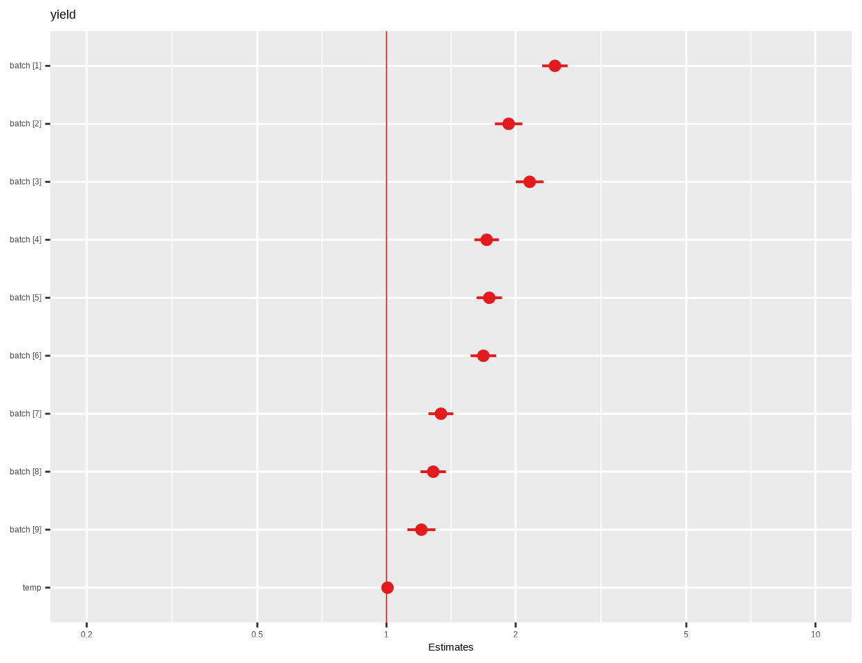
plot_model() function of {sjPlot} package creates plots the estimates from logistic model:

Code

plot_model(fit.beta.03, vline.color = "red")

Code

performance::performance(fit.beta.03)

# Indices of model performance

AIC      |     AICc |      BIC |    R2 |  RMSE | Sigma
------------------------------------------------------
-168.310 | -151.889 | -150.721 | 0.985 | 0.012 | 1.262

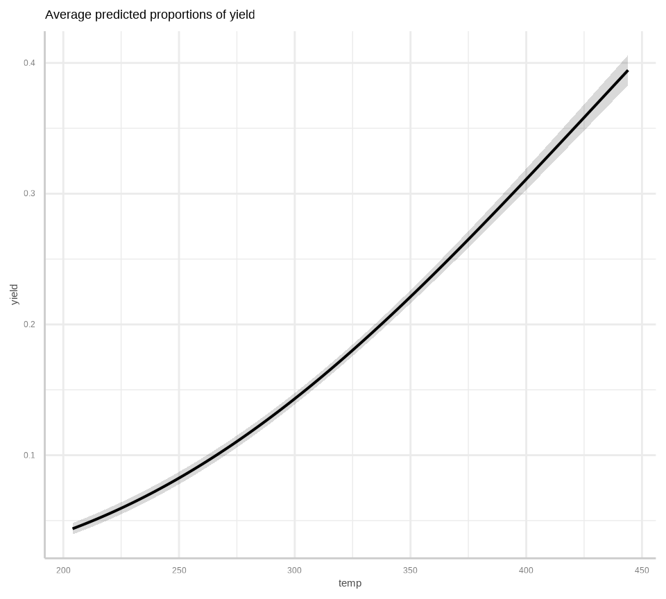
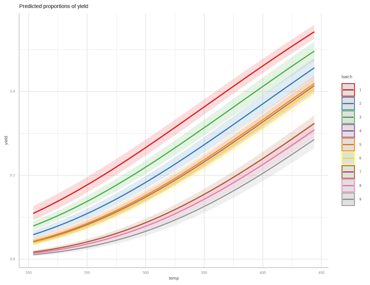
Marginal Effect

To calculate marginal effects and adjusted predictions, the predict_response() function of {ggeffects} package is used. This function can return three types of predictions, namely, conditional effects, marginal effects or marginal means, and average marginal effects or counterfactual predictions. You can set the type of prediction you want by using the margin argument.

Code

effect.temp<-ggeffects::predict_response(fit.beta.03, "temp", margin = "empirical")
plot(effect.temp)

Code

effect.temp.batch<-ggeffects::predict_response(fit.beta.03, terms = c("temp", "batch[1:9]"))
plot(effect.temp.batch)

Cross-validation

We’ll use 5-fold cross-validation to evaluate the model’s predictive performance using the Mean Squared Error (MSE) as the metric.

Code

cross_validate_betareg <- function(GasolineYield, k = 5) {
  n <- nrow(GasolineYield)
  indices <- sample(1:n)  # Randomize row indices
  fold_size <- floor(n / k)
  
  mse_values <- numeric(k)  # To store MSE for each fold
  
  for (i in 1:k) {
    # Create training and validation sets for the ith fold
    val_indices <- indices[((i - 1) * fold_size + 1):(i * fold_size)]
    train_data <- GasolineYield[-val_indices, ]
    val_data <- GasolineYield[val_indices, ]
    
    # Fit the model on the training set
    model <- betareg(yield ~ temp + batch,  link = "loglog", data = train_data)
    
    # Predict on the validation set
    predictions <- predict(model, newdata = val_data, type = "response")
    
    # Calculate MSE for this fold
    mse_values[i] <- mean((val_data$yield - predictions)^2)
  }
  
  # Return average MSE across all folds
  avg_mse <- mean(mse_values)
  return(avg_mse)
}

set.seed(123)
k <- 5
avg_mse_cv <- cross_validate_betareg(GasolineYield, k)
cat("Average Cross-Validated MSE:", avg_mse_cv, "\n")

Average Cross-Validated MSE: 0.0003569149

Summary and Conclusion

Beta regression is a powerful tool for modeling bounded continuous data, especially when the dependent variable takes values between 0 and 1, such as proportions or rates. By using the beta distribution, beta regression handles the constraints of bounded data while also providing flexibility in modeling both the mean and the dispersion of the response variable. In this tutorial, we demonstrated how to implement beta regression from scratch in R using maximum likelihood estimation to estimate the model parameters. Although this approach does not use specialized beta regression packages, it highlights the underlying statistical principles of beta regression, including the formulation of the log-likelihood function and optimization techniques.

By understanding the mechanics of beta regression, users can effectively apply this technique to their datasets with bounded response variables, providing more accurate and meaningful predictions compared to traditional linear regression.

8. Beta Regression

Overview

Beta Regression Model from Scratch

Generate Synthetic Data

Define the Beta Regression Log-Likelihood Function

Fit the Model Using Numerical Optimization

Display Model Summary

Dispersion Parameter

Evaluate Model Performance

Cross-validation

Beta Regression in R

Install Required R Packages

Load R-packages

Data

Fit Beta Models in R

Standard Beta Regression Model

Variable Dispersion Beta Regression Model

The Beta Regression with loh-log link function

The Beta Regression with link.phi = "log" link function

Model Comparison

Marginal Effect

Cross-validation

Summary and Conclusion

References

The Beta Regression with `loh-log` link function

The Beta Regression with `link.phi = "log"` link function