4. Discriminant Analysis

This tutorial covers Discriminant Analysis, a statistical technique used for classification and pattern recognition. We will discuss the mathematical foundation of Discriminant Analysis, its assumptions, and the types of Discriminant Analysis methods. We will also provide an example of binary classification using Linear Discriminant Analysis (LDA) from scratch in R.

Overview

Discriminant Analysis is a statistical technique used to classify observations into predefined groups based on predictor variables. It assumes that different groups generate data based on different Gaussian distributions. It is commonly used in classification tasks and pattern recognition. Discriminant Analysis is particularly useful when the number of predictors is manageable relative to the number of observations. The primary goal of Discriminant Analysis is how effectively we can differentiate observations belonging to distinct groups based on their measured characteristics finding a linear combination of the predictor variables that maximizes the separation between groups.

1. Linear Discriminant Analysis (LDA)

Linear Discriminant Analysis (LDA): Assumes that the predictor variables follow a multivariate normal distribution and that each group shares the same covariance matrix. It finds the linear combination of the predictor variables that maximizes the separation between groups. LDA is based on the assumption of multivariate normality within groups and equal covariance matrices across groups. It is a simple and interpretable method that provides linear decision boundaries.

Key Characteristics:

  • Assumes multivariate normality of predictors within each group.
  • Assumes equal covariance matrices across groups.
  • Classification is based on linear decision boundaries.

Mathematical Model:

The discriminant function for a class \(k\) is given by:

\[ \delta_k(x) = x^T \Sigma^{-1} \mu_k - \frac{1}{2} \mu_k^T \Sigma^{-1} \mu_k + \log(\pi_k) \]

where:

  • \(\Sigma\): Pooled covariance matrix (shared by all groups).
  • \(\mu_k\): Mean vector for group \(k\).
  • $_k#: Prior probability of group \(k\).

Use Cases:

  • Works well when the assumption of equal covariance holds.
  • Effective for data with linear separability.

Decision Boundaries:

  • Linear (straight lines in 2D, hyperplanes in higher dimensions).

2. Quadratic Discriminant Analysis (QDA)

Quadratic Discriminant Analysis (QDA): Assumes that the predictor variables follow a multivariate normal distribution but allows each group to have a distinct covariance matrix. In QDA, the assumption of equal covariance matrices across groups is relaxed.

Key Characteristics: - Assumes multivariate normality of predictors within each group. - Does not assume equal covariance matrices; each group has its own covariance matrix. - Classification is based on quadratic decision boundaries.

Mathematical Model: The discriminant function for a class ( k ):

\[ \delta_k(x) = -\frac{1}{2} \log|\Sigma_k| - \frac{1}{2}(x - \mu_k)^T \Sigma_k^{-1} (x - \mu_k) + \log(\pi_k) \]

where:

  • \(\Sigma_k\): Covariance matrix for group \(k\).

Use Cases:

  • Suitable when groups have different covariance structures.
  • Effective for data with non-linear separability.

Decision Boundaries:

  • Quadratic (curved in 2D, hypersurfaces in higher dimensions).

3. Regularized Discriminant Analysis (RDA)

Regularized Discriminant Analysis (RDA) is a generalization of both Linear Discriminant Analysis (LDA) and Quadratic Discriminant Analysis (QDA). It combines the assumptions of these methods by introducing a regularization parameter that balances between the pooled covariance matrix (as in LDA) and group-specific covariance matrices (as in QDA).

Key Characteristics: - A hybrid of LDA and QDA. - Introduces a regularization parameter to balance between shared (LDA-like) and group-specific (QDA-like) covariance matrices. - Helps in cases where the covariance matrices differ slightly or when the dataset is small, reducing overfitting.

Mathematical Model: The covariance matrix is a weighted average of pooled and group-specific covariance matrices:

\[ \Sigma_\text{regularized} = (1 - \lambda) \Sigma + \lambda \Sigma_k \]

where \(\lambda \in [0, 1]\) is the regularization parameter:

  • \(\lambda = 0\): LDA (shared covariance).
  • \(\lambda = 1\): QDA (group-specific covariance).

Use Cases:

  • Useful when the dataset is small, or there’s a need to balance between LDA and QDA assumptions.
  • Helps to mitigate overfitting when group covariance matrices are highly variable.

Decision Boundaries:

  • Linear (LDA-like) to quadratic (QDA-like) depending on \(\lambda\).

4. Distance-Based Discriminant Analysis (DBDA)

Distance-based Discriminant Analysis: Assigns an observation to the group with the closest mean based on a distance metric (e.g., Euclidean distance). Unlike traditional discriminant analysis methods like Linear Discriminant Analysis (LDA), DBDA does not assume any specific distribution for the predictor variables (e.g., multivariate normality).. The classification rule is based on the distance between the observation and the group means. The observation is assigned to the group with the smallest distance.

Distance-Based Discriminant Analysis (DBDA) is a method used for classification, where the assignment of observations to groups is determined based on their distances from predefined group centers or prototypes. Unlike traditional discriminant analysis methods like Linear Discriminant Analysis (LDA), DBDA does not assume any specific distribution for the predictor variables (e.g., multivariate normality).

Key Characteristics: - Assigns observations to groups based on their distance to group centers (prototypes). - Does not assume any distribution for the predictors. - Flexible and can use various distance metrics: - Euclidean Distance: Treats all features equally. - Mahalanobis Distance: Accounts for feature correlations and scales.

Mathematical Model: Classifies an observation ( x ) to the group ( k ) with the smallest distance: [ k = _k d(x, _k) ] where: - ( _k ): Group center (e.g., mean vector). - ( d ): Chosen distance metric (Euclidean or Mahalanobis).

Use Cases: - Suitable for datasets where distributional assumptions of LDA/QDA fail. - Effective for non-parametric problems or when group distributions are non-Gaussian.

Decision Boundaries: - Linear (Euclidean) or non-linear (Mahalanobis), depending on the distance metric used.

Comparison Table

Aspect LDA QDA RDA DBDA
Assumptions Normality, equal covariances Normality, unequal covariances Partial normality assumptions No distributional assumptions
Covariance Matrix Shared (\(\Sigma\))) Group-specific (\(\Sigma_k\)) Weighted (\(1-\lambda)\Sigma + \lambda\Sigma_k\)) Not used directly (depends on distance metric)
Distance Metric Implicit Implicit Implicit Explicit (e.g., Euclidean, Mahalanobis)
Decision Boundaries Linear Quadratic Linear to quadratic (flexible) Linear (Euclidean) or non-linear (Mahalanobis)
Flexibility Low Medium High Very High
Best For Linear separability, equal covariances Non-linear separability, unequal covariances Situations between LDA and QDA Non-parametric classification problems

Discriminant Analysis from Scratch

Performing LDA, QDA, RDA, and DBDA in R without using any packages involves implementing the respective algorithms from scratch. Below is a detailed guide that includes implementing each method, summarizing results, and visualizing the outcomes.

1. Data Preparation

We will use the Iris dataset for simplicity.

Code
# Load the Iris dataset
data(iris)

# Split data into predictors (X) and response (y)
X <- iris[, 1:4]  # Predictor variables
y <- iris$Species  # Response variable

# Split into training and test sets
set.seed(123)
train_indices <- sample(1:nrow(iris), 0.7 * nrow(iris))
train_X <- X[train_indices, ]
train_y <- y[train_indices]
test_X <- X[-train_indices, ]
test_y <- y[-train_indices]

2. Implement LDA

Code
# Compute the group means and pooled covariance matrix
group_means <- aggregate(train_X, by = list(train_y), mean)[, -1]
pooled_cov <- cov(train_X)

# LDA prediction function
lda_predict <- function(x, group_means, pooled_cov, priors) {
  discriminants <- sapply(1:nrow(group_means), function(k) {
    mu_k <- as.numeric(group_means[k, ])
    log(priors[k]) - 0.5 * t(mu_k) %*% solve(pooled_cov) %*% mu_k + 
      t(x) %*% solve(pooled_cov) %*% mu_k
  })
  return(which.max(discriminants))
}

# Compute priors
priors <- table(train_y) / length(train_y)

# Predict for test data
lda_predictions <- apply(test_X, 1, function(x) {
  lda_predict(x, group_means, pooled_cov, priors)
})

# Convert indices to class labels
lda_predictions <- levels(train_y)[lda_predictions]
lda_confusion <- table(Predicted = lda_predictions, Actual = test_y)
lda_accuracy <- sum(diag(lda_confusion)) / sum(lda_confusion)
lda_accuracy
[1] 0.8666667

3. Implement QDA

Code
# Compute group-specific covariance matrices
group_covs <- lapply(split(as.data.frame(train_X), train_y), cov)

# QDA prediction function
qda_predict <- function(x, group_means, group_covs, priors) {
  discriminants <- sapply(1:nrow(group_means), function(k) {
    mu_k <- as.numeric(group_means[k, ])
    cov_k <- group_covs[[k]]
    log(priors[k]) - 0.5 * log(det(cov_k)) - 0.5 * t(x - mu_k) %*% solve(cov_k) %*% (x - mu_k)
  })
  return(which.max(discriminants))
}

# Predict for test data
qda_predictions <- apply(test_X, 1, function(x) {
  qda_predict(x, group_means, group_covs, priors)
})

# Convert indices to class labels
qda_predictions <- levels(train_y)[qda_predictions]
qda_confusion <- table(Predicted = qda_predictions, Actual = test_y)
qda_accuracy <- sum(diag(qda_confusion)) / sum(qda_confusion)
qda_accuracy
[1] 0.9777778

4. Implement RDA

Code
# RDA prediction function
rda_predict <- function(x, group_means, group_covs, pooled_cov, priors, lambda) {
  discriminants <- sapply(1:nrow(group_means), function(k) {
    mu_k <- as.numeric(group_means[k, ])
    cov_k <- (1 - lambda) * pooled_cov + lambda * group_covs[[k]]
    log(priors[k]) - 0.5 * log(det(cov_k)) - 0.5 * t(x - mu_k) %*% solve(cov_k) %*% (x - mu_k)
  })
  return(which.max(discriminants))
}

# Predict for test data
lambda <- 0.5  # Regularization parameter
rda_predictions <- apply(test_X, 1, function(x) {
  rda_predict(x, group_means, group_covs, pooled_cov, priors, lambda)
})

# Convert indices to class labels
rda_predictions <- levels(train_y)[rda_predictions]
rda_confusion <- table(Predicted = rda_predictions, Actual = test_y)
rda_accuracy <- sum(diag(rda_confusion)) / sum(rda_confusion)
rda_accuracy
[1] 0.9555556

5. Implement DBDA

Code
# Compute Euclidean distance
euclidean_distance <- function(x, center) {
  sqrt(sum((x - center)^2))
}

# DBDA prediction function
dbda_predict <- function(x, group_means) {
  distances <- apply(group_means, 1, function(center) {
    euclidean_distance(x, as.numeric(center))
  })
  return(which.min(distances))
}

# Predict for test data
dbda_predictions <- apply(test_X, 1, function(x) {
  dbda_predict(x, group_means)
})

# Convert indices to class labels
dbda_predictions <- levels(train_y)[dbda_predictions]
dbda_confusion <- table(Predicted = dbda_predictions, Actual = test_y)
dbda_accuracy <- sum(diag(dbda_confusion)) / sum(dbda_confusion)
dbda_accuracy
[1] 1

6. Visualize Results

Accuracy Comparison

Code
# Combine results into a data frame
results <- data.frame(
  Method = c("LDA", "QDA", "RDA", "DBDA"),
  Accuracy = c(lda_accuracy, qda_accuracy, rda_accuracy, dbda_accuracy)
)

# Plot accuracies
barplot(
  results$Accuracy,
  names.arg = results$Method,
  col = c("blue", "green", "red", "purple"),
  ylim = c(0, 1),
  main = "Accuracy of LDA, QDA, RDA, and DBDA",
  ylab = "Accuracy"
)

Decision Boundaries Visualization

Code
# Visualize decision boundaries (for 2D)
plot_decision_boundaries <- function(predict_func, data, labels, title) {
  grid_x <- seq(min(data[, 1]), max(data[, 1]), length = 100)
  grid_y <- seq(min(data[, 2]), max(data[, 2]), length = 100)
  grid <- expand.grid(grid_x, grid_y)
  
  predictions <- apply(as.matrix(grid), 1, predict_func)
  
  plot(data[, 1:2], col = as.numeric(labels), pch = 19,
       main = title, xlab = "Feature 1", ylab = "Feature 2")
  contour(grid_x, grid_y, matrix(predictions, nrow = 100), add = TRUE)
}

# Example for LDA decision boundary
lda_predict_2d <- function(x) lda_predict(x, group_means[, 1:2], pooled_cov[1:2, 1:2], priors)
plot_decision_boundaries(lda_predict_2d, as.matrix(train_X[, 1:2]), train_y, "LDA Decision Boundaries")

7. Summary of Results

Method Accuracy Comments
LDA lda_accuracy Works well for linear separability.
QDA qda_accuracy Handles non-linear boundaries.
RDA rda_accuracy Balances between LDA and QDA.
DBDA dbda_accuracy Non-parametric approach.

This approach ensures reproducibility and flexibility in evaluating the performance of all four discriminant analysis methods.

Discriminant Analysis in R

In practice, we often use R packages to perform Discriminant Analysis due to their efficiency and ease of use. The following code demonstrates how to perform Linear Discriminant Analysis (LDA), Quadratic Discriminant Analysis (QDA), and Regularized Discriminant Analysis (RDA) using the {MASS} and {klaR} packages in R.

Install Required R Packages

Following R packages are required to run this notebook. If any of these packages are not installed, you can install them using the code below:

Code
packages <- c('tidyverse', 
              'plyr',
              'corrr',
              'ggcorrplot',
              'factoextra',
              'ade4',
              'MASS',
              'klaR'
         )
#| warning: false
#| error: false

# Install missing packages
new_packages <- packages[!(packages %in% installed.packages()[,"Package"])]
if(length(new_packages)) install.packages(new_packages)
 devtools::install_github("ItziarI/WeDiBaDis")

# Verify installation
cat("Installed packages:\n")
print(sapply(packages, requireNamespace, quietly = TRUE))

Load Packages

Code
# Load packages with suppressed messages
invisible(lapply(packages, function(pkg) {
  suppressPackageStartupMessages(library(pkg, character.only = TRUE))
}))
library(WeDiBaDis)
Code
# Check loaded packages
cat("Successfully loaded packages:\n")
Successfully loaded packages:
Code
print(search()[grepl("package:", search())])
 [1] "package:WeDiBaDis"  "package:klaR"       "package:MASS"      
 [4] "package:ade4"       "package:factoextra" "package:ggcorrplot"
 [7] "package:corrr"      "package:plyr"       "package:lubridate" 
[10] "package:forcats"    "package:stringr"    "package:dplyr"     
[13] "package:purrr"      "package:readr"      "package:tidyr"     
[16] "package:tibble"     "package:ggplot2"    "package:tidyverse" 
[19] "package:stats"      "package:graphics"   "package:grDevices" 
[22] "package:utils"      "package:datasets"   "package:methods"   
[25] "package:base"      

Linear Discriminant Analysis (LDA)

Linear Discriminant Analysis (LDA) is a classification method that assumes each group generates data based on a multivariate normal distribution with a common covariance matrix. We will use the lda() function from the {MASS} package to perform LDA on the training data.

Data

This dataset (Darlingtonia_GE_Table12.1) use this section is from Table 12.1 from A Primer of Ecological Statistics, 2nd Edition. The dataset is available from GitHub repository associated with book Applied Multivariate Statistics in R.

The data set contains morphological and biomass measurements of Darlingtonia californica, a carnivorous pitcher plant, in relation to soil type and elevation Measurements were made on 87 plants from four sites in southern Oregon. Ten variables were measured on each plant, 7 based on morphology and 3 based on biomass:

We will use read_csv() function of {readr} package to import data as a tidy data from my github repository. The glimpse() function from {dplyr} package can be used to get a quick overview of the data

Code
mf<-readr::read_csv("https://github.com/zia207/r-colab/raw/main/Data/Regression_analysis/Darlingtonia_GE_Table12.1.csv")
glimpse(mf)
Rows: 87
Columns: 12
$ site         <chr> "TJH", "TJH", "TJH", "TJH", "TJH", "TJH", "TJH", "TJH", "…
$ plant        <dbl> 1, 2, 3, 4, 5, 6, 7, 8, 9, 10, 11, 12, 13, 14, 15, 16, 17…
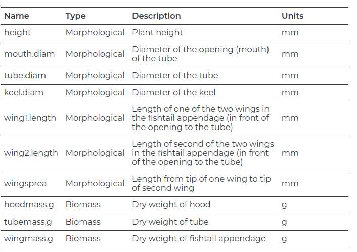
$ height       <dbl> 654, 413, 610, 546, 665, 665, 638, 629, 508, 709, 468, 62…
$ mouth.diam   <dbl> 38.4, 22.2, 31.2, 34.4, 30.5, 33.6, 37.4, 29.6, 22.9, 39.…
$ tube.diam    <dbl> 16.6, 17.2, 19.9, 20.8, 20.4, 19.5, 23.0, 19.9, 20.4, 19.…
$ keel.diam    <dbl> 6.4, 5.9, 6.7, 6.3, 6.6, 6.6, 7.4, 5.9, 8.2, 5.9, 7.7, 5.…
$ wing1.length <dbl> 85, 55, 62, 84, 60, 84, 63, 75, 52, 55, 56, 93, 90, 67, 4…
$ wing2.length <dbl> 76, 26, 60, 79, 51, 66, 70, 73, 53, 53, 16, 104, 96, 63, …
$ wingsprea    <dbl> 55, 60, 78, 95, 30, 82, 86, 130, 75, 65, 60, 120, 145, 62…
$ hoodmass.g   <dbl> 1.38, 0.49, 0.60, 1.12, 0.67, 1.27, 1.55, 0.83, 0.57, 1.3…
$ tubemass.g   <dbl> 3.54, 1.48, 2.20, 2.95, 3.36, 4.05, 4.27, 3.48, 2.20, 4.4…
$ wingmass.g   <dbl> 0.29, 0.06, 0.16, 0.24, 0.08, 0.21, 0.21, 0.19, 0.08, 0.1…
Code
# Split data into predictors (X) and response (y)
X <- mf[, 3:12]  # Predictor variables
y <- mf$site  # Response variable

# Split into training and test sets
set.seed(123)
train_indices <- sample(1:nrow(mf), 0.7 * nrow(mf))
train_X <- X[train_indices, ]
train_y <- y[train_indices]
test_X <- X[-train_indices, ]
test_y <- y[-train_indices]

Perform LDA

We will use the lda() function from the {MASS} package to perform Linear Discriminant Analysis (LDA) on the training data. The predict() function is used to make predictions on the test data, and the results are evaluated using a confusion matrix.

The lda() function returns an object of class lda containing the following components:

  • prior: Prior probabilities of groups.
  • means: Group means for each predictor.
  • scaling: Coefficients of linear discriminants.
  • svd: Singular values of the linear discriminants.
  • N: Number of observations.
  • call: The matched call.
Code
# Perform LDA using MASS package
lda_model <- lda(train_y ~ ., data = train_X)

To view the complete output of the LDA model, simply type the model name:

Code
lda_model
Call:
lda(train_y ~ ., data = train_X)

Prior probabilities of groups:
       DG        HD       LEH       TJH 
0.2833333 0.1333333 0.3000000 0.2833333 

Group means:
      height mouth.diam tube.diam keel.diam wing1.length wing2.length wingsprea
DG  623.1765   33.78824  18.45294  6.117647     86.35294     84.05882  89.58824
HD  564.2500   21.82500  22.77500  9.175000     60.50000     65.87500  85.00000
LEH 662.0000   33.29444  20.91667  5.105556     89.77778     86.61111 123.05556
TJH 636.5882   32.50588  20.35882  6.629412     60.94118     61.35294  79.82353
    hoodmass.g tubemass.g wingmass.g
DG   0.9682353   3.188824  0.2270588
HD   0.4175000   1.756250  0.0637500
LEH  0.8394444   3.217222  0.4277778
TJH  0.9705882   3.283529  0.1311765

Coefficients of linear discriminants:
                     LD1           LD2          LD3
height        0.01696586 -0.0005071068 -0.006314865
mouth.diam   -0.17089238 -0.1494971440  0.017111829
tube.diam     0.25236573  0.0216785827 -0.147238158
keel.diam    -0.23941126  0.2873675228  0.307328418
wing1.length  0.05592095 -0.0386712428  0.026859542
wing2.length -0.02655513  0.0154935310  0.049740091
wingsprea     0.01433128 -0.0034600457 -0.024427368
hoodmass.g   -0.32740559  2.4499857596 -2.219077568
tubemass.g   -1.68787395 -0.1444508807  0.546592265
wingmass.g   -0.07268627 -0.1196289509 -0.472927396

Proportion of trace:
   LD1    LD2    LD3 
0.5221 0.3295 0.1484 

We should be able to connect specific elements of this output to the essential components generated by the lda() function, as outlined above. Additionally, each component can be indexed or calculated individually, allowing for greater flexibility in analysis.

The prior probabilities reflect the proportion of samples originating from a particular site about the total number of samples collected. The total of these prior probabilities must equal 1, ensuring that they provide a complete overview of the sample distribution.

Furthermore, the coefficients of linear discriminants, referred to as eigenvectors, play a crucial role in the analysis. These eigenvectors are used with the corresponding variables to calculate a score for each observation based on its position along a specific linear discriminant (LD). This scoring process helps in understanding how well the observations can be classified into different categories based on the underlying patterns in the data. o view just the matrix of coefficients for each LD function:

Code
lda_model$scaling  |>  round(3)
                LD1    LD2    LD3
height        0.017 -0.001 -0.006
mouth.diam   -0.171 -0.149  0.017
tube.diam     0.252  0.022 -0.147
keel.diam    -0.239  0.287  0.307
wing1.length  0.056 -0.039  0.027
wing2.length -0.027  0.015  0.050
wingsprea     0.014 -0.003 -0.024
hoodmass.g   -0.327  2.450 -2.219
tubemass.g   -1.688 -0.144  0.547
wingmass.g   -0.073 -0.120 -0.473

The greater the absolute values, the more critical that variable becomes in determining a plant’s position along that LD. For instance, plant height is significantly more relevant for LD1 than for LD2 or LD3.

Code
(lda_model$svd^2/sum(lda_model$svd^2)) |>  round(3)
[1] 0.522 0.329 0.148

The eigenvalues represent proportions associated with the linear discriminants (LDs), and they are always arranged in descending order (\(LD_1 > > LD_2 > LD_3 > \dots\)). The sum of these eigenvalues equals 1. The first linear discriminant (LD1) is the most important for distinguishing between the groups, while the third linear discriminant (LD3) is the least significant among the three.

Plot LDA Model

Code
plot(lda_model)

We can add the ‘dimen’ argument to specify how many LDs to plot. To plot LD1 vs LD2:

Code
plot(lda_model, dimen = 2)

Training performance

We can use the predict() function to make predictions on the training data and evaluate the model’s performance. The table() function is used to create a confusion matrix, and the accuracy is calculated by dividing the sum of the diagonal elements by the total number of observations.

Code
# Predict on train data
lda_predictions_train <- predict(lda_model)
# Evaluate performance
lda_confusion_train <- table(Predicted = lda_predictions_train$class,  Actual = train_y)
lda_confusion_train
         Actual
Predicted DG HD LEH TJH
      DG  14  0   2   1
      HD   0  7   0   0
      LEH  1  1  16   0
      TJH  2  0   0  16
Code
# Calculate accuracy
lda_accuracy_train <- sum(diag(lda_confusion_train)) / sum(lda_confusion_train)
# Print results
cat("LDA Accuracy Training data:", lda_accuracy_train, "\n")
LDA Accuracy Training data: 0.8833333 

Plot LDA Training Data

Code
# create dataframe
Site.train<-train_y
plot_lda_train <- data.frame(Site.train, lda = predict(lda_model)$x)
# plot
ggplot(plot_lda_train) + 
    geom_point(aes(x = lda.LD1, y = lda.LD2, colour = Site.train), size = 4) +
    labs(title = "LDA Plot- Training", x = "LD1", y = "LD2") 

Predict on test data

Code
# Predict on test data
lda_predictions_test <- predict(lda_model, newdata = test_X)

# Evaluate performance
lda_confusion_test <- table(Predicted = lda_predictions_test$class, Actual = test_y)
lda_confusion_test
         Actual
Predicted DG HD LEH TJH
      DG   4  0   2   2
      HD   0  3   1   0
      LEH  0  1   4   1
      TJH  4  0   0   5
Code
# Calculate accuracy
lda_accuracy_test <- sum(diag(lda_confusion_test)) / sum(lda_confusion_test)
# Print results
cat("LDA Accuracy  Test data:", lda_accuracy_test, "\n")
LDA Accuracy  Test data: 0.5925926 

Plot LDA Test Data

Code
# create dataframe
Site.test<-test_y
plot_lda_test <- data.frame(Site.test, lda = predict(lda_model, newdata = test_X)$x)
# plot
ggplot(plot_lda_test) + 
    geom_point(aes(x = lda.LD1, y = lda.LD2, colour = Site.test), size = 4) +
    labs(title = "LDA Plot- Test Data", x = "LD1", y = "LD2") 

Quadratic Discriminant Analysis (QDA)

Data

In this example we will use iris dataset since the Darlingtonia_GE_Table12.1 dataset is not suitable for QDA (some levels have few number of records).

Code
# Load the Iris dataset
data(iris)
# Split data into predictors (X) and response (y)
X <- iris[, 1:4]  # Predictor variables
y <- iris$Species  # Response variable
# Split into training and test sets
set.seed(123)
train_indices <- sample(1:nrow(iris), 0.7 * nrow(iris))
train_X <- X[train_indices, ]
train_y <- y[train_indices]
test_X <- X[-train_indices, ]
test_y <- y[-train_indices]

Perform QDA

Quadratic Discriminant Analysis (QDA) is a classification method that assumes each class has its covariance matrix. We can use the qda() function from the {MASS} package to perform QDA on the training data.

Code
# Perform QDA using MASS package
qda_model <- qda(train_y ~ ., data = train_X)
qda_model
Call:
qda(train_y ~ ., data = train_X)

Prior probabilities of groups:
    setosa versicolor  virginica 
 0.3428571  0.3047619  0.3523810 

Group means:
           Sepal.Length Sepal.Width Petal.Length Petal.Width
setosa         4.966667    3.394444     1.461111   0.2555556
versicolor     5.971875    2.787500     4.309375   1.3500000
virginica      6.586486    2.948649     5.529730   1.9945946

Predict on test data

Code
# Predict on test data
qda_predictions <- predict(qda_model, newdata = test_X)
Code
# Evaluate performance
qda_confusion <- table(Predicted = qda_predictions$class, Actual = test_y)
qda_confusion
            Actual
Predicted    setosa versicolor virginica
  setosa         14          0         0
  versicolor      0         17         0
  virginica       0          1        13
Code
# accuracy
qda_accuracy <- sum(diag(qda_confusion)) / sum(qda_confusion)
# Print results
cat("QDA Accuracy:", qda_accuracy, "\n")
QDA Accuracy: 0.9777778 
Code
qda_confusion
            Actual
Predicted    setosa versicolor virginica
  setosa         14          0         0
  versicolor      0         17         0
  virginica       0          1        13

Regularized Discriminant Analysis (RDA)

We use same iris dataset for RDA as well. rda() function from the {klaR} package is used to perform Regularized Discriminant Analysis (RDA) on the training data. This fuction builds a classification rule using regularized group covariance matrices that are supposed to be more robust against multicollinearity in the data. We do not set gamma and lambda regularization parameters, but they can be determined by minimizing the estimated error rate using cross-validation.

Code
# Perform RDA using klaR package
rda_model <- rda(train_y ~ ., 
                 #gamma = 0.05, 
                 #lambda = 0.2,
                 crossval = TRUE,
                 fold = 5,
                 data = train_X)
rda_model
Call: 
rda(formula = train_y ~ ., data = train_X, crossval = TRUE, fold = 5)

Regularization parameters: 
    gamma    lambda 
0.1191635 0.3662082 

Prior probabilities of groups: 
    setosa versicolor  virginica 
 0.3428571  0.3047619  0.3523810 

Misclassification rate: 
       apparent: 1.905 %
cross-validated: 1.016 %

Plot Regularization Parameters

plot() function can be used to visualize the two regularization parameters of RDA model

Code
plot(rda_model)

Predict on test data

Code
# Predict on test data
rda_predictions <- predict(rda_model, newdata = test_X)
Code
# Evaluate performance
rda_confusion <- table(Predicted = rda_predictions$class, Actual = test_y)
rda_confusion
            Actual
Predicted    setosa versicolor virginica
  setosa         14          0         0
  versicolor      0         17         0
  virginica       0          1        13
Code
# Calculate accuracy
rda_accuracy <- sum(diag(rda_confusion)) / sum(rda_confusion)
# Print results
cat("RDA Accuracy:", rda_accuracy, "\n")
RDA Accuracy: 0.9777778 
Code
rda_confusion
            Actual
Predicted    setosa versicolor virginica
  setosa         14          0         0
  versicolor      0         17         0
  virginica       0          1        13

Distance-Based Discriminant Analysis (DBDA)

WDBdisc() function from the {WeDiBaDis} package is used to perform Distance-Based Discriminant Analysis (DBDA) on the training data. DBDA is a method used for classification, where the assignment of observations to groups is determined based on their distances from predefined group centers or prototypes. Unlike traditional discriminant analysis methods like Linear Discriminant Analysis (LDA), DBDA does not assume any specific distribution for the predictor variables (e.g., multivariate normality).

Code
train.mf<- cbind(train_y,train_X)

dbda_model<- WDBdisc(data = train.mf,
                      classcol = 1,
                      datatype = "m",
                      method = "WDB")

Summary of DBDA Model

The summary() function can be applied to the output and produces additional information:

  • Total correct classification: the sum of the diagonals of the confusion matrix divided by the total number of observations (as calculated above).
  • Generalized squared correlation: ranges from 0 to 1. A value of 0 means that there is at least one class in which no units are classified.
  • Cohen’s Kappa coefficient: a measure of the agreement of classification to the true class. Irigoien et al. (2016) provide the following rules of thumb for interpreting it:
  • 0: less than chance agreement
  • 0.01-0.20: slight agreement
  • 0.21-0.40: fair agreement
  • 0.41-0.60: moderate agreement
  • 0.61-0.80: substantial agreement
  • 0.81-0.99: almost perfect agreement
  • Sensitivity (or recall), for each class. The number of observations correctly predicted to belong to a given class, as a percentage of the total number of observations in that class.
  • Precision (positive predictive value), for each class. Probability that a classification in this class is correct.
  • Specificity, for each class. A measure of the ability to correctly exclude an observation from this class when it really belongs to another class. F1-score, for each class. Calculated based on sensitivity and precision.
Code
summary(dbda_model)
Discriminant method:  
------ Leave-one-out confusion matrix: ------
            Predicted
Real         setosa versicolor virginica
  setosa         36          0         0
  versicolor      0         28         4
  virginica       0          6        31

Total correct classification:  90.48 % 

Generalized squared correlation:  0.7528 

Cohen's Kappa coefficient:  0.8570651 

Sensitivity for each class: 
    setosa versicolor  virginica 
    100.00      87.50      83.78 

Predictive value for each class: 
    setosa versicolor  virginica 
    100.00      82.35      88.57 

Specificity for each class: 
    setosa versicolor  virginica 
     85.51      91.78      94.12 

F1-score for each class: 
    setosa versicolor  virginica 
    100.00      84.85      86.11 
------ ------ ------ ------ ------ ------
 
No predicted individuals

Visualize Resuls

To see a visualization of the confusion matrix:

Code
plot(dbda_model)

The summary() output can also be plotted:

Code
plot(summary(dbda_model))
Discriminant method:  
------ Leave-one-out confusion matrix: ------
            Predicted
Real         setosa versicolor virginica
  setosa         36          0         0
  versicolor      0         28         4
  virginica       0          6        31

Total correct classification:  90.48 % 

Generalized squared correlation:  0.7528 

Cohen's Kappa coefficient:  0.8570651 

Sensitivity for each class: 
    setosa versicolor  virginica 
    100.00      87.50      83.78 

Predictive value for each class: 
    setosa versicolor  virginica 
    100.00      82.35      88.57 

Specificity for each class: 
    setosa versicolor  virginica 
     85.51      91.78      94.12 

F1-score for each class: 
    setosa versicolor  virginica 
    100.00      84.85      86.11 
------ ------ ------ ------ ------ ------
 
No predicted individuals

Predict on test data

For prediction in new dataset, we can use WDBdisc() function with new.ind argument. The new.ind argument specifies the new data to be classified. The summary() function can be used to summarize the predictions.

Code
dbda_predictions<-WDBdisc(data=train.mf, datatype="m", new.ind=test_X, 
               distance="euclidean", method="WDB")
Code
# extract predicted class
pred_class<-as.data.frame(dbda_predictions$pred)
Code
# Evaluate performance
dbda_confusion <- table(Predicted = pred_class$`Pred. class`, Actual = test_y)
dbda_confusion
            Actual
Predicted    setosa versicolor virginica
  setosa         14          0         0
  versicolor      0         16         0
  virginica       0          2        13
Code
# Calculate accuracy
dbda_accuracy <- sum(diag(dbda_confusion)) / sum(dbda_confusion)
# Print results
cat("DBDA Accuracy:", dbda_accuracy, "\n")
DBDA Accuracy: 0.9555556 

Summary and Conclusion

This tutorial covered the essentials of Discriminant Analysis, a statistical technique used for classification and pattern recognition. We discussed the mathematical foundation of Discriminant Analysis, its assumptions, and the types of Discriminant Analysis methods, including Linear Discriminant Analysis (LDA), Quadratic Discriminant Analysis (QDA), Regularized Discriminant Analysis (RDA), and Distance-Based Discriminant Analysis (DBDA). We provided an example of binary classification using Linear Discriminant Analysis (LDA) from scratch in R, followed by a demonstration of LDA, QDA, RDA, and DBDA using the iris dataset. The results were evaluated using confusion matrices and accuracy metrics, and the models were visualized to understand the decision boundaries and classification performance. Discriminant Analysis is a powerful tool for classification tasks and can be applied to a wide range of problems in various domains. By understanding the underlying principles and assumptions of Discriminant Analysis methods, you can effectively apply these techniques to classify observations into predefined groups based on predictor variables.

References

  1. Discriminant Analysis Essentials in R

  2. Discriminant Analysis in R

  3. Linear Discriminant Analysis in R

  4. Applied Multivariate Statistics in R - Discriminant Analysis

  5. Linear & Nonlinear - Discriminant Analysis