![]()

Regularized Generalized Linear Model
Introduction to Regularized GLM
A Regularized Generalized Linear Model (GLM) extends the traditional GLM framework by incorporating regularization techniques to prevent overfitting and improve model generalization. Regularization is particularly useful when dealing with high-dimensional data or when the model is prone to overfitting due to multicollinearity, complex interactions, or a limited number of observations relative to the number of predictors.
Optimization of the Generalized Linear Model (GLM) refers to the process of finding the best set of coefficients that minimize the loss function. The loss function quantifies the difference between the predicted values and the actual values in the training data. In the context of regularized GLMs, the loss function includes a penalty term that discourages large coefficients, thereby preventing overfitting.
Generalized Linear Models (GLM) Overview
In a standard GLM, the model assumes that the outcome \(y\) is drawn from an exponential family distribution (e.g., normal, binomial, Poisson). The relationship between the predictor variables \(\mathbf{X}\) and the expected value of \(y\) is defined through a link function \(g\) as follows:
\[ g(\mathbb{E}[y]) = \mathbf{X} \beta \]
where:
- \(\mathbf{X}\) is the design matrix containing \(p\) predictor variables,
- \(\beta\)) is the vector of coefficients.
The likelihood function for GLM coefficients \(\beta\) is maximized to estimate the parameters.
Regularization in GLM
In a Regularized GLM, the model includes a penalty term to the objective function, which discourages large coefficient values and prevents overfitting. Two common types of regularization are Lasso (L1) and Ridge (L2) regularization:
Lasso (L1) Regularization: This adds a penalty proportional to the sum of the absolute values of the coefficients. Lasso encourages sparsity, meaning it often shrinks some coefficients to exactly zero. The objective function for Lasso regularization is given by:
\[ \text{minimize} \quad - \log L(\beta) + \lambda \sum_{j=1}^{p} |\beta_j| \]
Ridge (L2) Regularization: This adds a penalty proportional to the sum of the squared values of the coefficients. Ridge tends to shrink coefficients uniformly rather than pushing them to zero. The objective function for Ridge regularization is:
\[ \text{minimize} \quad - \log L(\beta) + \lambda \sum_{j=1}^{p} \beta_j^2 \]
Elastic Net Regularization: Elastic Net is a combination of Lasso and Ridge regularization, balancing both L1 and L2 penalties. It’s especially useful when there are correlated predictors. The objective function for Elastic Net is:
\[ \text{minimize} \quad - \log L(\beta) + \lambda_1 \sum_{j=1}^{p} |\beta_j| + \lambda_2 \sum_{j=1}^{p} \beta_j^2 \]
# Objective Function with Regularization
The objective function with regularization combines the primary goal of the model (such as minimizing error or maximizing likelihood) with a penalty term to discourage overfitting. This penalty imposes constraints on the model’s parameters, typically to ensure simplicity, prevent large coefficients, or enforce sparsity.
For a Generalized Linear Model (GLM), the regularized objective function can be written as:
\[ \text{minimize} \quad - \log L(\beta) + \lambda P \]
where:
- \(-\log L(\beta)\) is the negative log-likelihood for the GLM,
- \(\beta\) is the regularization penalty (e.g., L1, L2, or a combination),
- \(\lambda\) is the regularization parameter that controls the strength of the penalty.
The regularization parameter \(\lambda\) is typically chosen through cross-validation to optimize the model’s performance on unseen data.
Optimization of the Generalized Linear Model (GLM)
Optimization of the Generalized Linear Model (GLM) refers to the process of finding the best set of coefficients that minimize the loss function. The loss function quantifies the difference between the predicted values and the actual values in the training data. In the context of regularized GLMs, the loss function includes a penalty term that discourages large coefficients, thereby preventing overfitting. In regularized GLM, we typically aim to find the parameters that maximize the likelihood function, but we also want to avoid overfitting by applying a penalty (regularization). Let’s break down three common optimization techniques for regularized GLMs: Maximum Likelihood Estimation (MLE), Gradient Descent (GD), and Coordinate Descent. Each of these techniques can be used to fit regularized GLMs, with regularization terms like Lasso (L1), Ridge (L2), and Elastic Net.
1. Maximum Likelihood Estimation (MLE)
Maximum Likelihood Estimation (MLE) is a fundamental method used in statistical modeling to estimate the parameters of a model. In the context of GLMs, the goal is to maximize the likelihood of observing the data given a set of model parameters (coefficients).
For a GLM:
Given the data {\(X, y\)}, where \(X\) is the matrix of feature vectors and \(y\) is the vector of responses, we want to estimate the coefficients \(\beta\) that maximize the likelihood function \(L(\beta)\).
For a GLM with logistic regression (binary outcome), the likelihood is:
\[ L(\beta) = \prod_{i=1}^{n} P(y_i | X_i, \beta) = \prod_{i=1}^{n} \left(\frac{1}{1 + e^{-X_i \beta}}\right)^{y_i} \left(1 - \frac{1}{1 + e^{-X_i \beta}}\right)^{1 - y_i} \]
The log-likelihood is the natural log of this function:
\[ \log L(\beta) = \sum_{i=1}^{n} \left[ y_i \log(\sigma(X_i \beta)) + (1 - y_i) \log(1 - \sigma(X_i \beta)) \right] \]
where \(\sigma(z) = \frac{1}{1 + e^{-z}}\) is the logistic function.
Regularized MLE:
In regularized GLMs, we add a penalty term to the log-likelihood to avoid overfitting. For example:
- Ridge (L2 regularization): \(R(\beta) = \lambda \sum_{j=1}^{p} \beta_j^2\)
- Lasso (L1 regularization): \(R(\beta) = \lambda \sum_{j=1}^{p} |\beta_j|\)
- Elastic Net: A combination of L1 and L2 regularization.
Thus, the regularized log-likelihood becomes:
\[ \log L(\beta) - R(\beta) = \sum_{i=1}^{n} \left[ y_i \log(\sigma(X_i \beta)) + (1 - y_i) \log(1 - \sigma(X_i \beta)) \right] - \lambda R(\beta) \]
The goal is to maximize this objective function with respect to \(\beta\). In practice, this maximization is typically done numerically, since there is no closed-form solution when regularization is applied.
2. Gradient Descent (GD)
Gradient Descent is a first-order optimization algorithm that iteratively adjusts the parameters in the direction of the steepest decrease of the objective function. This is used to minimize a loss function, which in the case of regularized GLMs includes both the log-likelihood and the regularization term.
Steps in Gradient Descent:
The objective function for regularized GLMs is the negative log-likelihood plus the regularization term.
\[ \mathcal{L}(\beta) = -\log L(\beta) + \lambda R(\beta) \]
where \(L(\beta)\) is the likelihood function, and \(R(\beta)\) is the regularization term.
Gradient: We compute the gradient (the derivative) of the objective function with respect to the parameters \(\beta\):
\[ \nabla \mathcal{L}(\beta) = -\frac{1}{n} \sum_{i=1}^{n} X_i^T (y_i - \sigma(X_i \beta)) + \lambda \nabla R(\beta) \]
where \(\sigma(X_i \beta)\) is the logistic function, and \(\nabla R(\beta)\) is the gradient of the regularization term (e.g., \(\nabla R(\beta)\) = \(2\beta\) for Ridge and \(\nabla R(\beta) = \text{sign}(\beta)\) for Lasso).
Update Rule: Using the gradient, we update the parameters in the direction of the negative gradient:
\[ \beta^{(t+1)} = \beta^{(t)} - \eta \nabla \mathcal{L}(\beta^{(t)}) \]
where \(\eta\) is the learning rate that determines the size of each step.
Variants:
- Batch Gradient Descent: Uses the entire dataset to compute the gradient.
- Stochastic Gradient Descent (SGD): Uses one sample at a time to compute the gradient, which can be more efficient for large datasets.
- Mini-batch Gradient Descent: A compromise between Batch GD and SGD, using a small random subset of the data to compute the gradient.
Pros:
- Flexibility: Works with any regularization term (L1, L2, or Elastic Net).
- Scalability: Works well for large datasets, especially with SGD.
Cons:
- Slow Convergence: Can take many iterations to converge, especially if the learning rate is not chosen well.
- Requires tuning: Needs careful tuning of the learning rate and regularization parameter \(\lambda\).
3. Coordinate Descent
Coordinate Descent is an optimization algorithm that updates one parameter (or coordinate) at a time, while keeping all other parameters fixed. This method is particularly efficient for models with Lasso (L1) regularization and is used to solve the Lasso regression problem, which involves sparse solutions (many coefficients becoming zero).
Steps in Coordinate Descent:
The objective function for regularized GLMs is the same as in Gradient Decent
\[ \mathcal{L}(\beta) = -\log L(\beta) + \lambda R(\beta) \]
with the goal to minimize the negative log-likelihood and apply regularization.
In Coordinate Descent, we update one coefficient at a time, while holding the others fixed. The update rule for each coefficient \(\beta_j\) is:
\[ \beta_j^{(t+1)} = \text{soft-threshold}( \hat{\beta}_j, \lambda) \]
where \(\hat{\beta}_j\) is the coefficient obtained by solving the subproblem for \(\beta_j\), and soft-thresholding is used for Lasso (L1 penalty):
\[ \text{soft-threshold}(z, \lambda) = \text{sign}(z) \cdot \max(|z| - \lambda, 0) \]
This operation shrinks the coefficient \(\beta_j\) toward zero, and forces it to zero if the magnitude is smaller than \(\lambda\).
Update: For each coordinate \(j\) , we compute the residuals and update \(\beta_j\) to minimize the objective with respect to that coordinate.
Pros:
- Efficiency: Especially efficient for Lasso (L1 regularization) and Elastic Net.
- Sparsity: It leads to sparse solutions where many coefficients become exactly zero (important for feature selection).
- Simple to implement.
Cons:
- Inefficient for Ridge: Coordinate Descent is not as efficient for Ridge (L2) regularization since it doesn’t exploit the closed-form solution.
- Convergence Speed: It may take many iterations to converge, especially when the coefficients are not sparse or the regularization is small.
Summary Comparison of the Methods:
| Method | Description | Best For | Pros | Cons |
|---|---|---|---|---|
| Maximum Likelihood Estimation (MLE) | Maximizes the likelihood function, adding regularization as a penalty term | Logistic regression, GLMs in general | Provides the most statistically sound estimates | No closed-form solution with regularization, computationally expensive |
| Gradient Descent (GD) | Iterative optimization using the gradient of the objective function | General GLMs with regularization | Flexible for various regularization terms | Can be slow, requires tuning of learning rate |
| Coordinate Descent | Updates coefficients one by one, often used for Lasso (L1) | Lasso, Elastic Net | Efficient for sparse models, leads to sparse solutions | Slow for Ridge, needs many iterations for convergence |
Benefits of Regularized GLM
Regularized GLMs provide several advantages:
- Improved Generalization: By penalizing large coefficients, regularized GLMs tend to generalize better to new data.
- Handling Multicollinearity: Regularization can stabilize estimates when predictors are highly correlated.
- Sparse Solutions: L1 regularization promotes sparsity, which can result in simpler models by setting some coefficients to zero, making interpretation easier.
Regularized GLMs are a powerful tool for modeling complex data, especially in high-dimensional settings, by balancing model complexity with predictive performance.
In machine learning, a loss function is a mathematical function that measures the difference between the predicted output of a model and the actual output given a set of input data. The loss function quantifies how well the model performs and provides a way to optimize the model’s parameters during training.
The goal of machine learning is to minimize the loss function, which represents the error between the predicted output of the model and the actual output. By minimizing the loss function, the model learns to make better predictions on new data that it has not seen before.
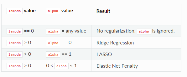
The following table describes the type of penalized model that results based on the values specifed for the lambda and alpha options.
Regularized GLM Models in R
In R, the {glmnet} package provides a powerful and efficient way to fit Regularized Generalized Linear Models (GLMs) for different types of outcomes, including Gaussian, logistic, multinomial, and Poisson models. It specializes in Lasso (L1) and Ridge (L2) regularization techniques, making it an ideal tool for dealing with high-dimensional data where the number of predictors exceeds the number of observations or when multicollinearity poses a challenge.
![]()
This package offers efficient algorithms for fitting penalized regression models, including the elastic net - a combination of Lasso and Ridge regression. Additionally, {glmnet} provides functions for cross-validation to identify the best regularization parameter and for extracting fitted model coefficients. “glmnet” is widely used in fields such as machine learning, statistics, and data science. It is an excellent choice for feature selection, prediction, and variable importance assessment tasks.
When working with {glmnet}, users can utilize various arguments to adjust the fitting process to their needs. This flexibility allows for a more tailored approach to the analysis and can lead to more accurate results. To help with this customization, we have outlined some of the most commonly used arguments below. However, for a more comprehensive understanding of the {glmnet} package and its capabilities, we recommend referring to the official documentation by typing ?glmnet.
The glmnet() function, which is used for fitting generalized linear models with regularization (Lasso, Ridge, or Elastic Net), employs Coordinate Descent. optimization method.
glmnet(x, y, alpha = 1, lambda = NULL)x: matrix of predictor variablesy: the response or outcome variable, which is a binary variable.alphais for the elastic net mixing parameter α, with range \(α∈[0,1].α=1\) is lasso regression (default) and \(α=0\) is ridge regression.nlambdais the number of \(λ\) values in the sequence (default is 100).lambdacan be provided if the user wants to specify the lambda sequence, but typical usage is for the program to construct the lambda sequence on its own. When automatically generated, the \(λ\) sequence is determined bylambda.maxandlambda.min.ratio. The latter is the ratio of smallest value of the generated \(λ\) sequence (saylambda.min) tolambda.max. The program generatesnlambdavalues linear on the log scale fromlambda.maxdown tolambda.min.lambda.maxis not user-specified but is computed from the input \(x\) and \(y\): it is the smallest value forlambdasuch that all the coefficients are zero. Foralpha = 0(ridge)lambda.maxwould be \(∞\): in this case we pick a value corresponding to a small value foralphaclose to zero.)standardizeis a logical flag forxvariable standardization prior to fitting the model sequence. The coefficients are always returned on the original scale. Default isstandardize = TRUE.
K-fold cross-validation can be performed using the cv.glmnet function. In addition to all the glmnet parameters, cv.glmnet has its special parameters including nfolds (the number of folds), (user-supplied folds), and type.measure (the loss used for cross-validation): `” or “mse” for squared loss, and
maeuses mean absolute error.alphais for the elastic net mixing parameterα, with range \(α∈[0,1].α=1\) is lasso regression (default) and \(α=0\) is ridge regression.“1”: for lasso regression
“0”: for ridge regression
a value between 0 and 1 (say 0.3) for elastic net regression.
Step-by-Step Guide
Install and Load the glmnet Package
install.packages("glmnet")
library(glmnet)
**Prepare the Data
The
glmnetpackage expects the predictor matrix \(X\) and response vector \(y\) in a specific format:- \(X\): A matrix (not a data frame) of predictor variables.
- $ y$: A vector (or factor for classification) of the response variable.
# Example of creating matrix format data
X <- as.matrix(your_dataframe[, -ncol(your_dataframe)])  # predictors
y <- your_dataframe$response_variable  # response
Fitting Different Types of Regularized GLMs
glmnetfits models using both Lasso (L1) and Ridge (L2) regularization, controlled by thealphaparameter:alpha = 1: Lasso regressionalpha = 0: Ridge regression0 < alpha < 1: Elastic Net, a mixture of L1 and L2 regularization
Regularized GLMs for Different Distributions
1. Gaussian Model (Linear Regression)
For a continuous response variable, use the family = "gaussian" option:
# Gaussian model (Linear Regression)
fit_gaussian <- glmnet(X, y, family = "gaussian", alpha = 1)  # Lasso regularization
# Alternatively, use alpha = 0 for Ridge or alpha = 0.5 for Elastic Net
2. Logistic Regression (Binary Classification)
For binary classification, use the family = "binomial" option:
# Logistic model (Binary Classification)
fit_logistic <- glmnet(X, y, family = "binomial", alpha = 1)  # Lasso regularization
3. Multinomial Model (Multi-Class Classification)
For a categorical response with more than two classes, use family = "multinomial":
# Multinomial model (Multi-Class Classification)
fit_multinomial <- glmnet(X, y, family = "multinomial", alpha = 1)  # Lasso regularization
4. Poisson Model (Count Data)
For count data, use the family = "poisson" option:
# Poisson model (Count Data)
fit_poisson <- glmnet(X, y, family = "poisson", alpha = 1)  # Lasso regularization
Cross-Validation to Select Optimal Lambda
The cv.glmnet function performs cross-validation to find the optimal value of \(\lambda\)), the regularization parameter. This ensures the best balance between bias and variance.
# Cross-validation for the Gaussian model
cv_fit_gaussian <- cv.glmnet(X, y, family = "gaussian", alpha = 1)
best_lambda_gaussian <- cv_fit_gaussian$lambda.min  # Optimal lambda value

# Cross-validation for the Logistic model
cv_fit_logistic <- cv.glmnet(X, y, family = "binomial", alpha = 1)
best_lambda_logistic <- cv_fit_logistic$lambda.min

# Cross-validation for the Multinomial model
cv_fit_multinomial <- cv.glmnet(X, y, family = "multinomial", alpha = 1)
best_lambda_multinomial <- cv_fit_multinomial$lambda.min

# Cross-validation for the Poisson model
cv_fit_poisson <- cv.glmnet(X, y, family = "poisson", alpha = 1)
best_lambda_poisson <- cv_fit_poisson$lambda.min
Making Predictions
After determining the best ( ) value, you can use it to make predictions on new data:
# Predict on new data using the optimal lambda
new_X <- as.matrix(new_data[, -ncol(new_data)])  # Convert predictors to matrix

# Gaussian model prediction
pred_gaussian <- predict(cv_fit_gaussian, new_X, s = best_lambda_gaussian)

# Logistic model prediction
pred_logistic <- predict(cv_fit_logistic, new_X, s = best_lambda_logistic, type = "response")

# Multinomial model prediction
pred_multinomial <- predict(cv_fit_multinomial, new_X, s = best_lambda_multinomial, type = "response")

# Poisson model prediction
pred_poisson <- predict(cv_fit_poisson, new_X, s = best_lambda_poisson, type = "response")
Summary
By following this approach, you can perform regularized GLMs for Gaussian, logistic, multinomial, and Poisson models in R using the glmnet package. The regularization parameter \(\lambda\) is chosen through cross-validation to enhance model performance on unseen data.
Books
Here are some books related to the Regularized Generalized Linear Model:
- Generalized Linear Models - Taylor & Francis eBooks
- Generalized Linear Models (Chapman & Hall/CRC Monographs on Statistics)
- An Introduction to Generalized Linear Models - Taylor & Francis eBooks
These books provide comprehensive coverage of generalized linear models and their applications.