3.6. Generalized Additive Mixed Models (GAMMs)

Generalized Additive Mixed Models (GAMMs) are powerful tools for analyzing complex data structures, allowing for flexible modeling of non-linear relationships while accounting for random effects to handle hierarchical or grouped data. In R, the {mgcv} and {gamm4} packages offer robust and complementary approaches for fitting GAMMs. It bridge the gap between purely parametric models and fully non-parametric approaches, offering unparalleled flexibility and interpretability. By leveraging the capabilities of these packages, you can effectively model complex data patterns and gain insights into the relationships between variables in your data.

Overview

Generalized Additive Models (GAMs) and their mixed-effects counterpart, Generalized Additive Mixed Models (GAMMs), are advanced statistical techniques that expand upon the capabilities of generalized linear models. These models are particularly useful for capturing non-linear relationships between variables, allowing for greater flexibility in modeling complex data patterns. The GAMs are most useful when your data is independent, and you are focused solely on smooth, non-linear effects. In contrast, GAMMs are employed when your data is hierarchical, clustered, or involves repeated measures, enabling you to account for random effects in addition to smooth effects. For example, a GAM might model crop yield using smooth effects of temperature and rainfall. Alternatively, a GAMM would model crop yield by incorporating smooth effects and accounting for variability across different farms through random effects.

Key Differences Between GAM (Generalized Additive Model) and GAMM (Generalized Additive Mixed Model)

Feature	GAM (Generalized Additive Model)	GAMM (Generalized Additive Mixed Model)
Random Effects	Does not include random effects.	Includes random effects to account for grouped or hierarchical data structures.
Correlated Data	Assumes independence of observations.	Handles correlated data, such as repeated measures, through random effects.
Flexibility	Models only smooth, non-linear effects of predictors.	Combines smooth, non-linear effects with random effects to model both fixed and hierarchical/random structures.
Data Structure	Suitable for flat data (no clustering or hierarchical structure).	Suitable for hierarchical or clustered data (e.g., patients within hospitals, students within schools).
Formula Structure	Only includes smooth terms for predictors ($Y = f(X_1) + f(X_2)%). \| Combines smooth terms and random effects ($Y = f(X_1) + f(X_2) + $).
Computational Complexity	Relatively simpler and faster to compute.	More computationally intensive due to the estimation of random effects.
Example	Modeling non-linear relationships between temperature and crop yield.	Modeling non-linear relationships between temperature and crop yield, accounting for random effects like variability across regions.

Components of a GAMM include:

Response Variable ($Y$): The outcome variable, which can follow various distributions (e.g., Gaussian, Poisson, Binomial).
Fixed Effects: These capture the population-level effects of predictors.
Smooth Terms: These describe non-linear relationships between predictors and the response.
Random Effects: These capture variation due to grouping or hierarchical structures in the data.
Link Function: Relates the predictors to the response variable (e.g., log link for Poisson regression).

A GAMM can be written as:

\[ g(E[Y]) = \beta_0 + \sum_j f_j(X_j) + \mathbf{Z}b \]

where:

$g(\cdot)$: Link function.
$E[Y]$: Expected value of the response.
$\beta_0$: Intercept.
$f_j(X_j)$: Smooth functions of predictors $X_j$.
$\mathbf{Z}b$: Random effects with $b \sim N(0, \Sigma)$.

For example, you are studying tree growth in a forest. The dataset includes:

Response variable ($Y$): Tree height.
Fixed predictors: Temperature ($Temp$) and soil pH ($pH$).
Random effects: Variability due to location (different forest plots).
Smooth terms: Non-linear relationship between temperature and tree height.

The GAMM model cab be written as:

\[ \text{Height}_i = \beta_0 + f_1(Temp_i) + f_2(pH_i) + \text{RandomEffect}_{Plot} + \epsilon_in \] where:

$f_1(Temp_i)$ and $f_2(pH_i)$: Smooth functions capturing the non-linear effects of temperature and pH.
RandomEffect$_{Plot}$: Accounts for differences in tree growth across forest plots.
$\epsilon_i$: Residual error.

*Advantages of GAMMs 1. Flexibility in modeling complex, non-linear relationships. 2. Ability to incorporate random effects for grouped or correlated data. 3. Applicability to a wide range of response variable types.

When to Use GAMMs

Longitudinal or hierarchical data with non-linear effects.
Ecological studies, where natural processes often exhibit non-linear relationships.
Epidemiological studies with clustered data (e.g., patients nested in hospitals).

Install Required R Packages

Following R packages are required to run this notebook. If any of these packages are not installed, you can install them using the code below:

Code

packages <- c('tidyverse',
              'DataExplorer',
              'sjPlot',
              'gam',
              'gamair',
              'mgcv',
              'gamlss',
              'gratia',
              'latticeExtra',
              'gamm4',
              'agridat',
              'itsadug'
              )

#| warning: false
#| error: false

# Install missing packages
new_packages <kages[!(packages %in% installed.packages()[,"Package"])]
if(length(new_packages)) install.packages(new_packages)

# Verify installation
cat("Installed packages:\n")
print(sapply(packages, requireNamespace, quietly = TRUE))

Load Packages

Code

# Load packages with suppressed messages
invisible(lapply(packages, function(pkg) {
  suppressPackageStartupMessages(library(pkg, character.only = TRUE))
}))

Code

# Check loaded packages
cat("Successfully loaded packages:\n")

Successfully loaded packages:

Code

print(search()[grepl("package:", search())])

 [1] "package:itsadug"       "package:plotfunctions" "package:agridat"      
 [4] "package:gamm4"         "package:lme4"          "package:Matrix"       
 [7] "package:latticeExtra"  "package:lattice"       "package:gratia"       
[10] "package:gamlss"        "package:parallel"      "package:gamlss.dist"  
[13] "package:gamlss.data"   "package:mgcv"          "package:nlme"         
[16] "package:gamair"        "package:gam"           "package:foreach"      
[19] "package:splines"       "package:sjPlot"        "package:DataExplorer" 
[22] "package:lubridate"     "package:forcats"       "package:stringr"      
[25] "package:dplyr"         "package:purrr"         "package:readr"        
[28] "package:tidyr"         "package:tibble"        "package:ggplot2"      
[31] "package:tidyverse"     "package:stats"         "package:graphics"     
[34] "package:grDevices"     "package:utils"         "package:datasets"     
[37] "package:methods"       "package:base"

Generalized Additive Mixed Models (GAMM) in R

In this exercise we will learn how to fit Generalized Additive Mixed Models (GAMM) in R using the gamm4 package. GAMMs are an extension of Generalized Additive Models (GAMs) that allow for the inclusion of random effects in the model. This makes them particularly useful for analyzing data with a hierarchical structure, such as repeated measures or clustered data. In this tutorial, we will walk through the process of fitting a GAMM in R using the {gamm4} package, including specifying the model formula, fitting the model, and interpreting the results. The {gamm4} is based on gamm from package {mgcv}, but uses {lme4} rather than {nlme} as the underlying fitting engine. The {gamm4} is more robust numerically than {gamm}, and by avoiding PQL gives better performance for binary and low mean count data. Its main disadvantage is that it can not handle most multi-penalty smooths (i.e. not te type tensor products or adaptive smooths).

Data

In this exercise, we will use the lasrosas.corn dataset from the {agridat} package. This dataset contains information on corn yield and various environmental factors from a field experiment conducted in Las Rosas, Argentina with variable N application. The dataset includes the following variables:

year: year of the experiment, 1999 or 2001

lat: latitude

long: longitude

yield: corn yield, quintals/ha

nitro: nitrogen fertilizer, kg/ha

topo: topographic factor

bv: brightness value (proxy for low organic matter content)

rep: blocking factor

nf: nitrogen as a factor, N0-N4

Code

mf = lasrosas.corn  
glimpse(mf)

Rows: 3,443
Columns: 9
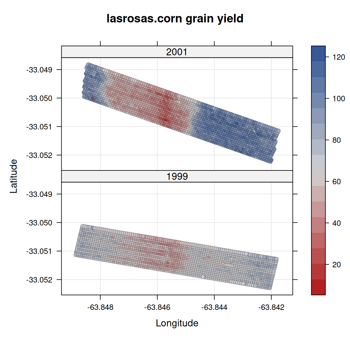
$ year  <int> 1999, 1999, 1999, 1999, 1999, 1999, 1999, 1999, 1999, 1999, 1999…
$ lat   <dbl> -33.05113, -33.05115, -33.05116, -33.05117, -33.05118, -33.05120…
$ long  <dbl> -63.84886, -63.84879, -63.84872, -63.84865, -63.84858, -63.84851…
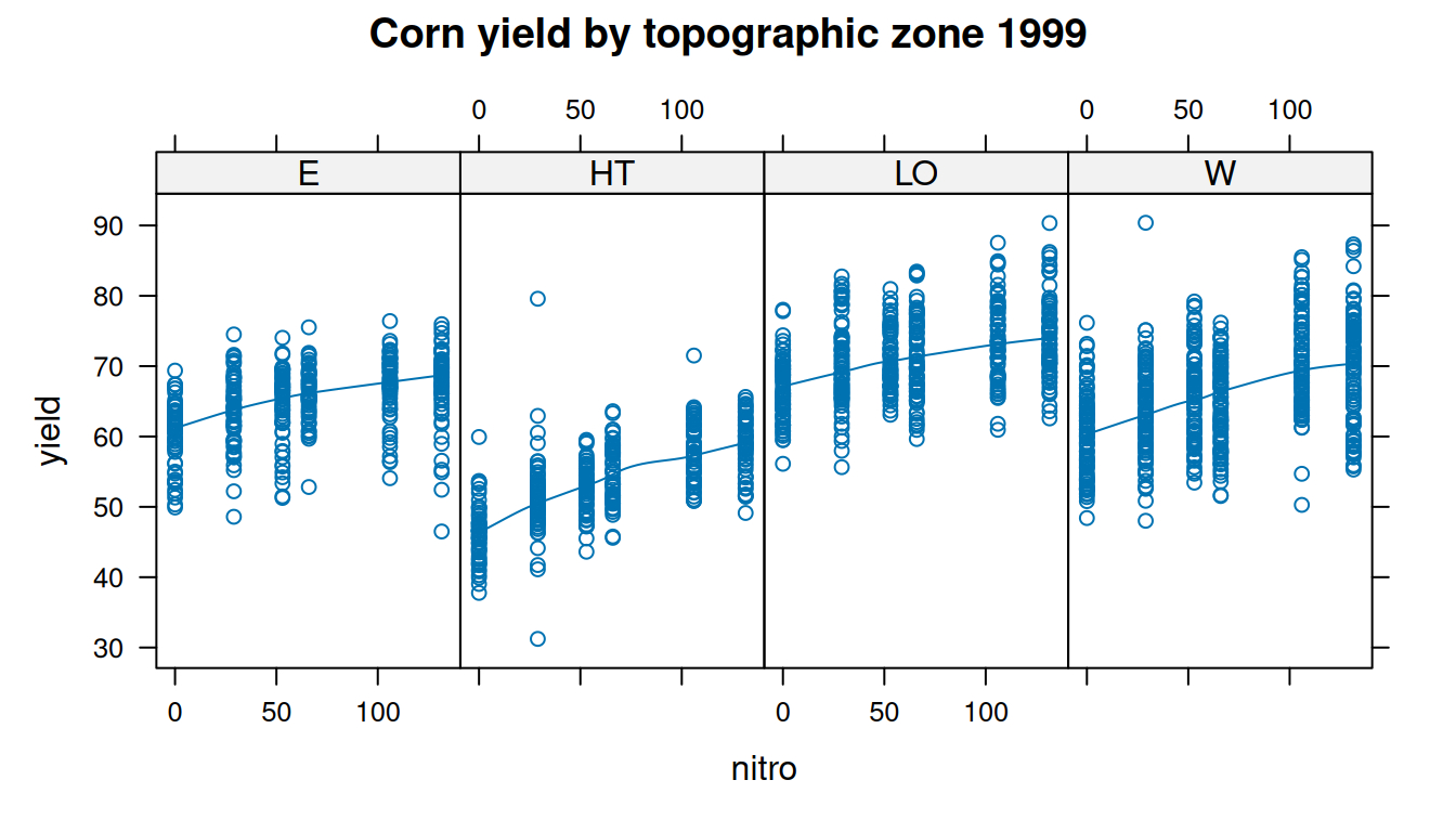
$ yield <dbl> 72.14, 73.79, 77.25, 76.35, 75.55, 70.24, 76.17, 69.17, 69.77, 6…
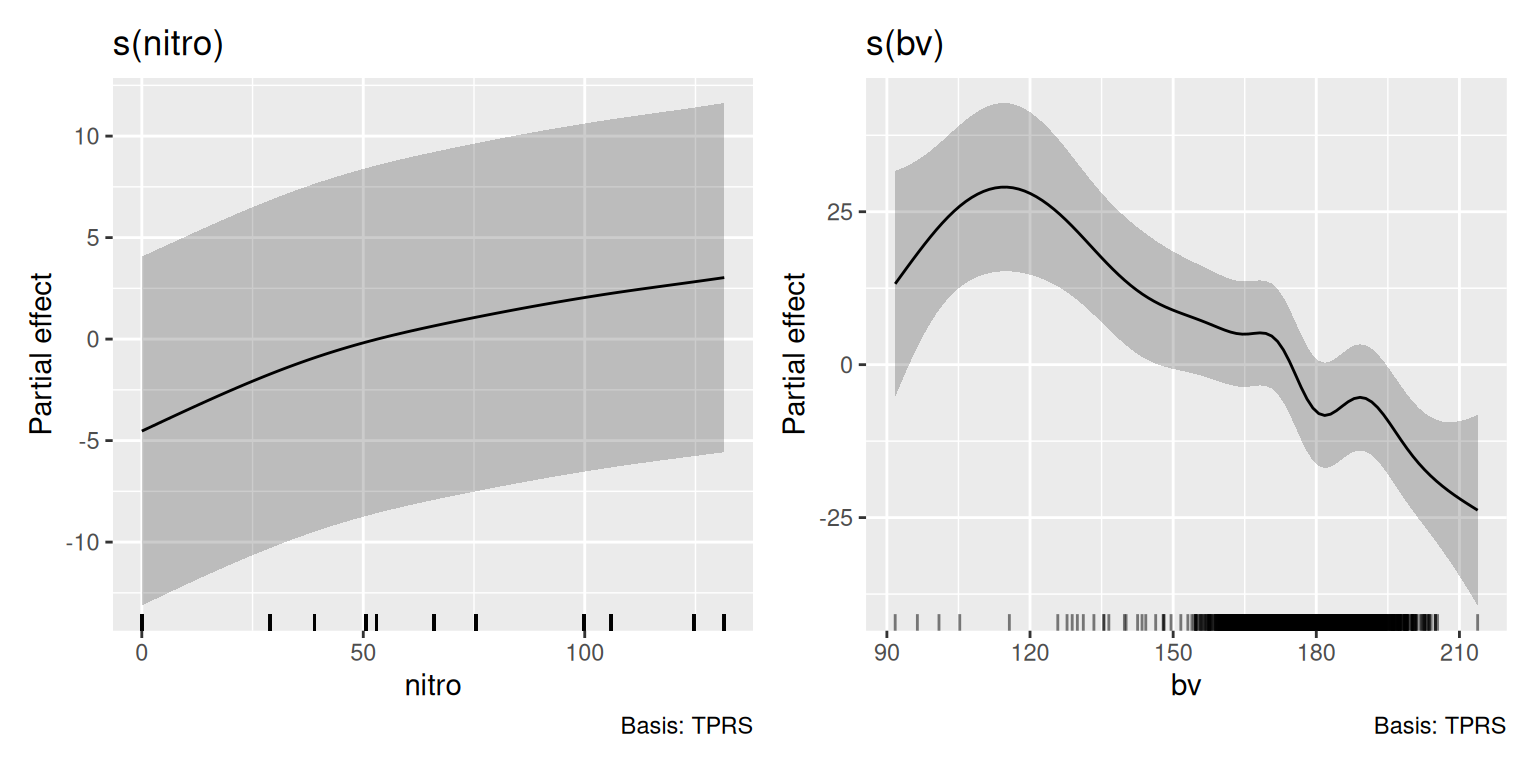
$ nitro <dbl> 131.5, 131.5, 131.5, 131.5, 131.5, 131.5, 131.5, 131.5, 131.5, 1…
$ topo  <fct> W, W, W, W, W, W, W, W, W, W, W, W, W, W, W, W, W, W, W, W, W, W…
$ bv    <dbl> 162.60, 170.49, 168.39, 176.68, 171.46, 170.56, 172.94, 171.86, …
$ rep   <fct> R1, R1, R1, R1, R1, R1, R1, R1, R1, R1, R1, R1, R1, R1, R1, R1, …
$ nf    <fct> N5, N5, N5, N5, N5, N5, N5, N5, N5, N5, N5, N5, N5, N5, N5, N5, …

Exploratory Data Analysis

First we will visualize the data using scatter plots and maps to explore the relationships between the variables in 4 topographic zones.

Code

# A quadratic response to nitrogen is suggested
d1 <- subset(mf, year==1999)
xyplot(yield~nitro|topo, data=d1, type=c('p','smooth'), layout=c(4,1),
       main="Corn yield by topographic zone 1999")

Code

# A quadratic response to nitrogen is suggested
d2 <- subset(mf, year==2001)
xyplot(yield~nitro|topo, data=d1, type=c('p','smooth'), layout=c(4,1),
       main="Corn yield by topographic zone 2001")

Then, we will create a scatterplot matrix to visualize the relationships between the variables in the lasrosas.corn dataset.

Code

# yield map
libs(lattice,latticeExtra)  # for panel.levelplot.points
redblue <- colorRampPalette(c("firebrick", "lightgray", "#375997"))
levelplot(yield ~ long*lat|factor(year), data=mf, 
          main="lasrosas.corn grain yield", xlab="Longitude", ylab="Latitude",
          scales=list(alternating=FALSE),
          prepanel = prepanel.default.xyplot,
          panel = panel.levelplot.points,
          type = c("p", "g"), aspect = "iso", col.regions=redblue)

Fit GAMM with {mgcv} Package

In the {mgcv} package in R, you can fit a Generalized Additive Mixed Model (GAMM) with different smoothing functions using the gamm() function. By specifying different smooth terms (e.g., s() for thin plate regression splines, te() for tensor product smooths, ti() for tensor interactions, and bs="cr" for cubic regression splines), you can experiment with various types of smooths.

"tp": Thin plate regression spline (default).
"cr": Cubic regression spline.
"ps": P-spline.
"cs": Cyclic cubic regression spline, suitable for cyclic data (e.g., periodic).
te(x, z): Tensor product smooth for interactions of multiple covariates.

GAMM with One Random Intercept

In this example, we’ll fit a GAMM model using the gamm() function to model the relationship between the yield variable and nitro, topo, and bv and year with random intercept. The gamm() function call {lme} in the normal errors identity link case, or by a call to {gammPQL} (a modification of {gammPQL} from the {MASS} library) otherwise. In the latter case estimates are only approximately MLEs. The routine is typically slower than gam, and not quite as numerically robust.

We’ll use a cubic regression spline with 3 degrees of freedom for bv and nitro variables. We will use s() is the shorthand for fitting smoothing splines in gamm() function.

Code

# Fit the GAMM with random intercepts 
gamm_intercept_01 <- gamm(yield ~ s(nitro) + s(bv) + topo, random=list(year=~1), data = mf)
summary(gamm_intercept_01)

    Length Class Mode
lme 18     lme   list
gam 31     gam   list

gamm() returns a list with two items:

lme: the fitted model object returned by lme or gammPQL. Note that the model formulae and grouping structures may appear to be rather bizarre, because of the manner in which the GAMM is split up and the calls to lme and gammPQL are constructed.

Code

summary(gamm_intercept_01$lme)

Linear mixed-effects model fit by maximum likelihood
  Data: strip.offset(mf) 
       AIC      BIC    logLik
  27045.92 27107.36 -13512.96

Random effects:
 Formula: ~Xr - 1 | g
 Structure: pdIdnot
              Xr1       Xr2       Xr3       Xr4       Xr5       Xr6       Xr7
StdDev: 0.7188879 0.7188879 0.7188879 0.7188879 0.7188879 0.7188879 0.7188879
              Xr8
StdDev: 0.7188879

 Formula: ~Xr.0 - 1 | g.0 %in% g
 Structure: pdIdnot
           Xr.01    Xr.02    Xr.03    Xr.04    Xr.05    Xr.06    Xr.07    Xr.08
StdDev: 169.2563 169.2563 169.2563 169.2563 169.2563 169.2563 169.2563 169.2563

 Formula: ~1 | year %in% g.0 %in% g
        (Intercept) Residual
StdDev:    6.162527 12.15998

Fixed effects:  y ~ X - 1 
                 Value Std.Error   DF   t-value p-value
X(Intercept)  77.26658  4.385804 3436  17.61742  0.0000
XtopoHT      -24.65428  0.737647 3436 -33.42285  0.0000
XtopoLO        3.48653  0.670062 3436   5.20330  0.0000
XtopoW        -8.76205  0.622251 3436 -14.08122  0.0000
Xs(nitro)Fx1   2.83462  0.696258 3436   4.07122  0.0000
Xs(bv)Fx1     -2.87206  4.113063 3436  -0.69828  0.4851
 Correlation: 
             X(Int) XtopHT XtopLO XtopoW Xs(n)F1
XtopoHT      -0.073                             
XtopoLO      -0.071  0.360                      
XtopoW       -0.077  0.467  0.413               
Xs(nitro)Fx1  0.000  0.002 -0.012  0.001        
Xs(bv)Fx1     0.001  0.000 -0.006 -0.014  0.006 

Standardized Within-Group Residuals:
        Min          Q1         Med          Q3         Max 
-4.24285801 -0.79553419  0.01105193  0.77851425  3.30504525 

Number of Observations: 3443
Number of Groups: 
                   g           g.0 %in% g year %in% g.0 %in% g 
                   1                    1                    2

gam: an object of class gam, less information relating to GCV/UBRE model selection. At present this contains enough information to use predict, summary and print methods and vis.gam, but not to use e.g. the anova method function to compare models. This is based on the working model when using gammPQL.

Code

summary(gamm_intercept_01$gam)


Family: gaussian 
Link function: identity 

Formula:
yield ~ s(nitro) + s(bv) + topo

Parametric coefficients:
            Estimate Std. Error t value Pr(>|t|)    
(Intercept)  77.2666     4.3845  17.623  < 2e-16 ***
topoHT      -24.6543     0.7374 -33.433  < 2e-16 ***
topoLO        3.4865     0.6699   5.205 2.06e-07 ***
topoW        -8.7621     0.6221 -14.085  < 2e-16 ***
---
Signif. codes:  0 '***' 0.001 '**' 0.01 '*' 0.05 '.' 0.1 ' ' 1

Approximate significance of smooth terms:
           edf Ref.df     F p-value    
s(nitro) 2.366  2.366 60.70  <2e-16 ***
s(bv)    8.391  8.391 64.01  <2e-16 ***
---
Signif. codes:  0 '***' 0.001 '**' 0.01 '*' 0.05 '.' 0.1 ' ' 1

R-sq.(adj) =  0.527   
  Scale est. = 147.87    n = 3443

The {gratia} package is designed to work with {mgcv} and offers enhanced visualization and diagnostic tools.

Code

# Enhanced visualization
gratia::draw(gamm_intercept_01$gam) # Generates nicely formatted plots

GAMM with Multiple Random Effects

In this example, we’ll fit a GAMM model with two random components year and topo using the gamm() function. We will use a cubic regression spline with 3 degrees of freedom for bv and nitro variables. We will use s() is the shorthand for fitting smoothing splines in gamm() function.

Code

#|error: false
#|warning: false
# Fit the GAMM with random intercepts 
gamm_intercept_02 <- gamm(yield ~ s(nitro) + s(bv),  random=list(year=~1, year=~topo), data = mf)

Warning in lme.formula(y ~ X - 1, random = rand, data = strip.offset(mf), : nlminb problem, convergence error code = 1
  message = iteration limit reached without convergence (10)

Code

summary(gamm_intercept_02$lme)

Linear mixed-effects model fit by maximum likelihood
  Data: strip.offset(mf) 
       AIC      BIC    logLik
  25364.53 25468.98 -12665.27

Random effects:
 Formula: ~Xr - 1 | g
 Structure: pdIdnot
              Xr1       Xr2       Xr3       Xr4       Xr5       Xr6       Xr7
StdDev: 0.7762645 0.7762645 0.7762645 0.7762645 0.7762645 0.7762645 0.7762645
              Xr8
StdDev: 0.7762645

 Formula: ~Xr.0 - 1 | g.0 %in% g
 Structure: pdIdnot
          Xr.01   Xr.02   Xr.03   Xr.04   Xr.05   Xr.06   Xr.07   Xr.08
StdDev: 110.578 110.578 110.578 110.578 110.578 110.578 110.578 110.578

 Formula: ~1 | year %in% g.0 %in% g
         (Intercept)
StdDev: 1.365002e-19

 Formula: ~topo | year %in% year %in% g.0 %in% g
 Structure: General positive-definite, Log-Cholesky parametrization
            StdDev    Corr                
(Intercept) 21.335251 (Intr) topoHT topoLO
topoHT      31.762934 -0.995              
topoLO       4.315866  0.855 -0.901       
topoW       16.086436 -0.987  0.968 -0.763
Residual     9.489345                     

Fixed effects:  y ~ X - 1 
                Value Std.Error   DF   t-value p-value
X(Intercept) 62.38699 0.2680759 3439 232.72138  0.0000
Xs(nitro)Fx1  3.02228 0.6737756 3439   4.48558  0.0000
Xs(bv)Fx1    -2.83547 3.0924051 3439  -0.91691  0.3593
 Correlation: 
             X(Int) Xs(n)F1
Xs(nitro)Fx1  0.006        
Xs(bv)Fx1    -0.005  0.008 

Standardized Within-Group Residuals:
        Min          Q1         Med          Q3         Max 
-4.99791096 -0.51263385 -0.01384824  0.50816067  4.33477016 

Number of Observations: 3443
Number of Groups: 
                               g                       g.0 %in% g 
                               1                                1 
            year %in% g.0 %in% g year.1 %in% year %in% g.0 %in% g 
                               2                                2

Code

summary(gamm_intercept_02$gam)


Family: gaussian 
Link function: identity 

Formula:
yield ~ s(nitro) + s(bv)

Parametric coefficients:
            Estimate Std. Error t value Pr(>|t|)    
(Intercept)   62.387      0.268   232.8   <2e-16 ***
---
Signif. codes:  0 '***' 0.001 '**' 0.01 '*' 0.05 '.' 0.1 ' ' 1

Approximate significance of smooth terms:
           edf Ref.df     F p-value    
s(nitro) 2.736  2.736 89.82  <2e-16 ***
s(bv)    8.191  8.191 84.86  <2e-16 ***
---
Signif. codes:  0 '***' 0.001 '**' 0.01 '*' 0.05 '.' 0.1 ' ' 1

R-sq.(adj) =  0.239   
  Scale est. = 90.048    n = 3443

Model Comparison

Now we will compare the two models using the anova() function to see if the model with multiple random effects is significantly better than the model with a single random effect. Here we have use lme object from the gamm_intercept_01 and gamm_intercept_02 objects.

Code

anova(gamm_intercept_01$lme, gamm_intercept_02$lme)

                      Model df      AIC      BIC    logLik   Test  L.Ratio
gamm_intercept_01$lme     1 10 27045.92 27107.36 -13512.96                
gamm_intercept_02$lme     2 17 25364.53 25468.98 -12665.27 1 vs 2 1695.382
                      p-value
gamm_intercept_01$lme        
gamm_intercept_02$lme  <.0001

From above output we can see that the model with multiple random effects is significantly better than the model with a single random effect (p < 0.05), suggesting that the additional random effect improves the model fit.

We may use bam() function of {mgcv} package to fit both GAM and GAMM models. The bam() function uses a penalized likelihood approach (MEL), which can be more computationally efficient than the gamm() function for large datasets. The bam() function is particularly useful for fitting GAMs with random effects, as it can handle large datasets more efficiently than the gamm() function. The bam() function is similar to the gamm() function, but it uses a different fitting algorithm that can be more memory-efficient for large datasets. The bam() function can be used to fit GAMs with random effects by specifying the random-effect smooths in the model formula.

For example, we can use bam() function to fit a GAM without random-effect. The by parameter is used to the smooths separately for each level of the nominal variable of category of topo. The k parameter is used to specify the number of basis functions to use for the smooth. The s() function is used to define the smooths of nitro and bv with a cubic regression spline basis.

Code

bam_01 <- bam(yield ~ 
                s(nitro, by = topo,   k=9) +
                s(bv, k=9), 
                data= mf)
summary(bam_01)


Family: gaussian 
Link function: identity 

Formula:
yield ~ s(nitro, by = topo, k = 9) + s(bv, k = 9)

Parametric coefficients:
            Estimate Std. Error t value Pr(>|t|)    
(Intercept)  69.9745     0.2393   292.4   <2e-16 ***
---
Signif. codes:  0 '***' 0.001 '**' 0.01 '*' 0.05 '.' 0.1 ' ' 1

Approximate significance of smooth terms:
                  edf Ref.df      F  p-value    
s(nitro):topoE  7.921  7.998  42.72  < 2e-16 ***
s(nitro):topoHT 7.720  7.974  16.62  < 2e-16 ***
s(nitro):topoLO 7.948  7.999  64.72  < 2e-16 ***
s(nitro):topoW  1.732  2.131  14.85 7.65e-07 ***
s(bv)           6.405  7.321 317.61  < 2e-16 ***
---
Signif. codes:  0 '***' 0.001 '**' 0.01 '*' 0.05 '.' 0.1 ' ' 1

R-sq.(adj) =    0.5   Deviance explained = 50.5%
fREML =  14044  Scale est. = 196.63    n = 3443

We can use bam() fuction to fit a GAMM with random-effect smooths of s(year,bs="re") and s(topo, bs="re"). The first parameter is the random-effect factor, which is interpreted as a random intercept. This function is useful for very large datasets, as it uses a sparse matrix representation of the smooths, which can be more memory-efficient than the gamm() function.

Code

bam_02 <- bam(yield ~ 
                s(nitro, by = topo,   k=9) +
                s(bv, k=9) +  
                s(year,bs="re") +
                s(topo, bs="re"),
                data= mf)
summary(bam_02)


Family: gaussian 
Link function: identity 

Formula:
yield ~ s(nitro, by = topo, k = 9) + s(bv, k = 9) + s(year, bs = "re") + 
    s(topo, bs = "re")

Parametric coefficients:
            Estimate Std. Error t value Pr(>|t|)    
(Intercept)  -9830.3      486.2  -20.22   <2e-16 ***
---
Signif. codes:  0 '***' 0.001 '**' 0.01 '*' 0.05 '.' 0.1 ' ' 1

Approximate significance of smooth terms:
                   edf Ref.df      F p-value    
s(nitro):topoE  7.8824  7.995  27.12  <2e-16 ***
s(nitro):topoHT 7.9264  7.998  42.84  <2e-16 ***
s(nitro):topoLO 7.9257  7.998  41.25  <2e-16 ***
s(nitro):topoW  1.0004  1.001  51.36  <2e-16 ***
s(bv)           7.5295  7.930  75.68  <2e-16 ***
s(year)         0.9976  1.000 432.49  <2e-16 ***
s(topo)         2.9961  3.000 597.54  <2e-16 ***
---
Signif. codes:  0 '***' 0.001 '**' 0.01 '*' 0.05 '.' 0.1 ' ' 1

R-sq.(adj) =  0.699   Deviance explained = 70.3%
fREML =  13191  Scale est. = 118.26    n = 3443

Then, compare the two models using the compareML() function of {itsadyg} package to see if the model with random effects is significantly better than the model without random effects.

Code

compareML(bam_01, bam_02)

bam_01: yield ~ s(nitro, by = topo, k = 9) + s(bv, k = 9)

bam_02: yield ~ s(nitro, by = topo, k = 9) + s(bv, k = 9) + s(year, bs = "re") + 
    s(topo, bs = "re")

Chi-square test of fREML scores
-----
   Model    Score Edf Difference    Df  p.value Sig.
1 bam_01 14043.95  11                               
2 bam_02 13190.71  13    853.239 2.000  < 2e-16  ***

AIC difference: 1748.25, model bam_02 has lower AIC.

The results show that the model bam_03 is better since it has a lower AIC score. Therefore, it is better for us to include the random intercepts.

Fit GAMM with {gamm4} Package

The gamm4() function fits a GAMM model with random intercepts for the year variable. The random argument specifies the random effects to include in the model, in this case, a random intercept for the year variable. The s() function is used to specify the smooth terms for the nitro and bv variables.

Code

gamm4_01<- gamm4(yield ~ s(nitro) + s(bv)+ topo, random=~(1|year), data = mf)
summary(gamm4_01)

    Length Class   Mode
mer  1     lmerMod S4  
gam 32     gam     list

gam an object of class gam. At present this contains enough information to use predict, plot, summary and print methods and vis.gam, from package mgcv but not to use e.g. the anova method function to compare models.

Code

summary(gamm4_01$gam)


Family: gaussian 
Link function: identity 

Formula:
yield ~ s(nitro) + s(bv) + topo

Parametric coefficients:
            Estimate Std. Error t value Pr(>|t|)    
(Intercept)  77.2642     6.1841  12.494  < 2e-16 ***
topoHT      -24.6571     0.7374 -33.437  < 2e-16 ***
topoLO        3.4914     0.6699   5.212 1.98e-07 ***
topoW        -8.7561     0.6221 -14.075  < 2e-16 ***
---
Signif. codes:  0 '***' 0.001 '**' 0.01 '*' 0.05 '.' 0.1 ' ' 1

Approximate significance of smooth terms:
           edf Ref.df     F p-value    
s(nitro) 2.676  2.676 54.16  <2e-16 ***
s(bv)    8.408  8.408 63.95  <2e-16 ***
---
Signif. codes:  0 '***' 0.001 '**' 0.01 '*' 0.05 '.' 0.1 ' ' 1

R-sq.(adj) =  0.527   
lmer.REML =  27012  Scale est. = 148.02    n = 3443

mer: The fitted model object returned by lmer or glmer. Extra random and fixed effect terms will appear relating to the estimation of the smooth terms. Note that unlike lme objects returned by gamm, everything in this object always relates to the fitted model itself, and never to a PQL working approximation: hence the usual methods of model comparison are entirely legitimate.

Code

summary(gamm4_01$mer)

Linear mixed model fit by REML ['lmerMod']

REML criterion at convergence: 27012.2

Scaled residuals: 
    Min      1Q  Median      3Q     Max 
-4.2393 -0.7915  0.0124  0.7771  3.2963 

Random effects:
 Groups   Name        Variance  Std.Dev.
 Xr       s(nitro)    9.022e-01   0.9499
 Xr.0     s(bv)       2.970e+04 172.3340
 year     (Intercept) 7.606e+01   8.7212
 Residual             1.480e+02  12.1665
Number of obs: 3443, groups:  Xr, 8; Xr.0, 8; year, 2

Fixed effects:
             Estimate Std. Error t value
X(Intercept)  77.2642     6.1841  12.494
XtopoHT      -24.6571     0.7374 -33.437
XtopoLO        3.4914     0.6699   5.212
XtopoW        -8.7561     0.6221 -14.075
Xs(nitro)Fx1   2.9843     0.8394   3.555
Xs(bv)Fx1     -2.9353     4.1250  -0.712

Correlation of Fixed Effects:
            X(Int) XtopHT XtopLO XtopoW Xs(n)F1
XtopoHT     -0.051                             
XtopoLO     -0.050  0.360                      
XtopoW      -0.055  0.467  0.413               
Xs(nitr)Fx1  0.000  0.001 -0.012  0.003        
Xs(bv)Fx1    0.001  0.000 -0.006 -0.014  0.008

Summary and Conclusions

Generalized Additive Mixed Models (GAMMs) are powerful tools for analyzing complex data structures, allowing for flexible modeling of non-linear relationships while accounting for random effects to handle hierarchical or grouped data. The gamm() and bam() functions from the {mgcv} package is a versatile tool for fitting GAMMs with a wide range of smooth terms and random effects. The gamm4() function from the {gamm4} package provides a more robust and numerically stable alternative to gamm() for fitting GAMMs with random effects. By leveraging the capabilities of these packages, you can effectively model complex data patterns and gain insights into the relationships between variables in your data.

3.6. Generalized Additive Mixed Models (GAMMs)

Overview

Install Required R Packages

Load Packages

Generalized Additive Mixed Models (GAMM) in R

Data

Exploratory Data Analysis

Fit GAMM with {mgcv} Package

GAMM with One Random Intercept

GAMM with Multiple Random Effects

Model Comparison

Fit GAMM with {gamm4} Package

Summary and Conclusions

References