![]()

Survival Analysis
Survival analysis is a statistical method that examines the time until a specific event occurs, such as death, disease relapse, or machine failure. It is valuable for studying event timing and accounts for cases where some individuals do not experience the event during the study period, known as censoring. This chapter will cover the key concepts, functions, and types of survival analysis, along with their applications in different fields.
Introduction to Survial Analysis
Survival analysis is a branch of statistics that focuses on analyzing time-to-event data. It is commonly used to study the duration until a specific event occurs, such as time until death, disease relapse, or machine failure. This method is especially useful when the timing of the event is the primary concern, and it accounts for cases where some individuals may not experience the event during the study period, a situation known as censoring.
Key Concepts
Event: Survival Analysis typically focuses on time to event data. In the most general sense, it consists of techniques for positive-valued random variables, such as
time to death
time to onset (or relapse) of a disease
length of a contract
duration of a policy
money paid by health insurance
viral load measurements
time to finishing a master thesis
Survival Time: The time from the starting point (like diagnosis or study enrollment) to the event of interest. For individuals who don’t experience the event during the study, this time is considered censored.
Censoring: Occurs when the event of interest has not happened for some subjects during the observation period.
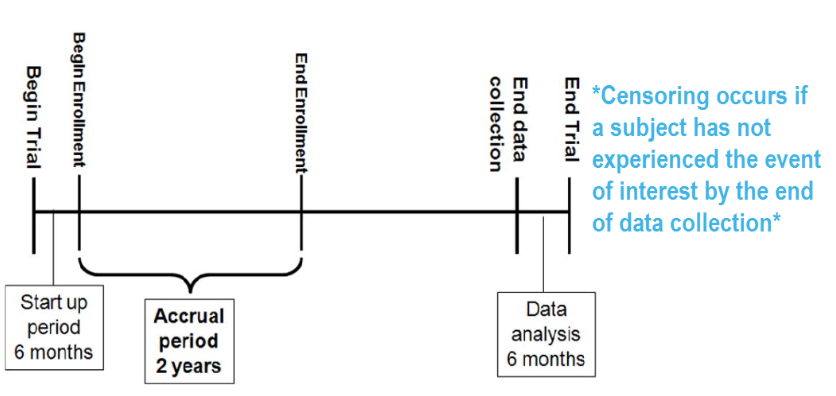 Note
NoteRICH JT, NEELY JG, PANIELLO RC, VOELKER CCJ, NUSSENBAUM B, WANG EW. A PRACTICAL GUIDE TO UNDERSTANDING KAPLAN-MEIER CURVES. Otolaryngology head and neck surgery: official journal of American Academy of Otolaryngology Head and Neck Surgery. 2010;143(3):331-336. doi:10.1016/j.otohns.2010.05.007.
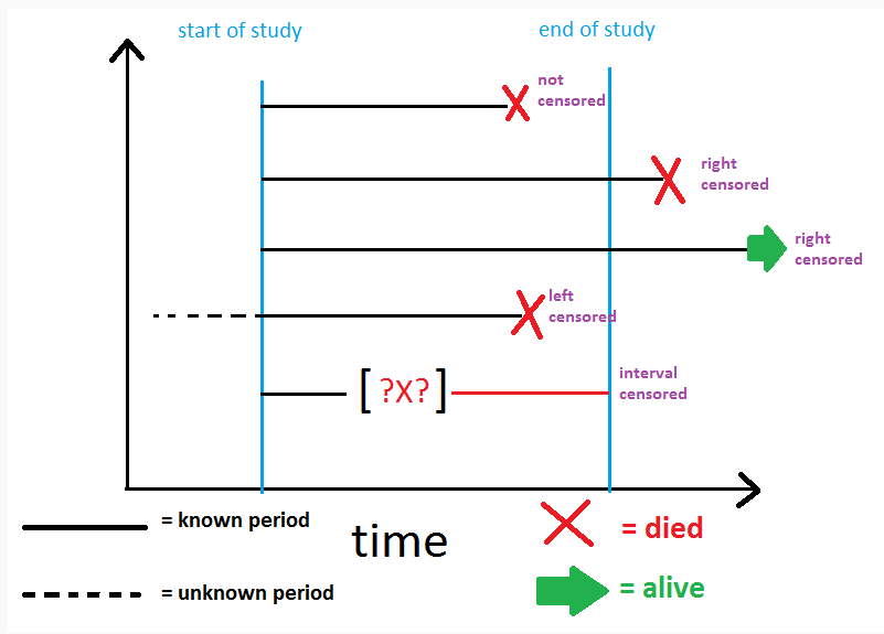
There are three common types:
Right censoring: The most common type, where the event hasn’t occurred by the end of the study, or the subject is lost to follow-up.
Left censoring: The event happened before the subject entered the study, but the exact time is unknown.
Interval censoring: The event happened within a certain interval, but the exact timing is unclear.
Functions Used in Survival Analysis
Survival Function \((S(t))\)
This gives the probability that the time to event is greater than some time \(t\).
Mathematically: \(S(t)=P(T>t)\)
It starts at 1 (all subjects are “surviving” at time \((0)\) and decreases over time.
Hazard Function \((h(t))\)
This describes the instantaneous rate at which events occur, given that the subject has survived up to time \(t\).
Mathematically: \(h(t)=\frac{f(t)}{S(t)}\), where \(f(t)\) is the probability density function of the event time.
It’s a measure of the event risk over time.
Cumulative Hazard Function \((H(t))\)
It sums the hazard over time, giving a total risk of experiencing the event by time \(t\).
Mathematically: \(H(t) = \int_0^t h(u) \, du\)
The survival function is generally considered to be smooth in a theoretical context; however, when examining real-world data, we find that events often occur at discrete points in time.
The survival probability, represented as \(S(t)\), indicates the likelihood of surviving beyond a particular time threshold. This probability is conditional upon the individual having survived up until that moment. To estimate this survival probability, we take the number of patients who remain alive and have not been lost to follow-up at that specific time and divide it by the total number of patients who were alive just prior to that time.
The Kaplan-Meier estimator provides a method to calculate the survival probability at any given time by multiplying these conditional probabilities from the start of the observation period up to that moment.
At the very beginning, or at time zero, the survival probability is set at 1, which implies that \(S(t_0) = 1\), indicating that all individuals are alive at the start of the study.ory, the survival function is smooth; in practice, we observe events on a discrete time scale.
The survival probability at a certain time, \(S(t)\), is a conditional probability of surviving beyond that time, given that an individual has survived just prior to that time. The survival probability can be estimated as the number of patients who are alive without loss to follow-up at that time, divided by the number of patients who were alive just prior to that time.
The Kaplan-Meier estimate of survival probability at a given time is the product of these conditional probabilities up until that given time.
At time 0, the survival probability is 1, i.e. \(S(t_0)=1\).
Types of Survival Analysis:
Here’s an overview of the different types of survival regression models:
1. Nonparametric Methods
Overview:
Nonparametric survival analysis involves techniques that make no assumptions about the underlying distribution of survival times. The most common non-parametric methods include the Kaplan-Meier estimator for estimating survival curves and the log-rank test for comparing survival between groups.
Kaplan-Meier estimate: The Kaplan-Meier estimate (also known as the Kaplan-Meier survival curve) is a non-parametric statistic used to estimate the survival function from time-to-event data, particularly in the presence of censored data. It provides an empirical survival curve that shows the probability of survival over time, often used in medical research to estimate survival probabilities and visualize the proportion of subjects surviving at different points in time
Key Features:
Does not require assumptions about the underlying distribution of survival times.
Plots survival curves to visualize survival probabilities over time.
Model Structure:
The Kaplan-Meier estimator calculates survival probabilities by dividing the study time into intervals and updating survival probability estimates each time an event occurs. The survival probability is calculated using the formula:
\[ S^(t)= \prod_{t_i \leq t} \left( \frac{n_i - d_i}{n_i} \right) \]
where:
\(n_i\) is the number of individuals at risk just before time \(t_1\).
\(d_i\) is the number of events (e.g., deaths) occurring at time \(t_i\).
The product of these terms across all event times gives the overall survival probability at any time \(t\)
When to use:
- To compare survival between two or more groups (e.g., patients receiving different treatments).
Log-Rank Test (Comparing Survival Curves)
Overview:
The log-rank test is a hypothesis test used to compare the survival distributions of two or more groups.
It evaluates whether there is a statistically significant difference between the survival curves.
Key Features:
Non-parametric test, used in conjunction with Kaplan-Meier curves.
Compares survival times across different strata (e.g., treatment groups).
Use Case:
- To determine if there is a difference in survival between two treatment groups in a clinical trial.
2. Cox Proportional-Hazards Model (Cox Regression)
Overview:
- The Cox proportional-hazards model is the most widely used survival regression model. It is semi-parametric, meaning it makes no assumptions about the baseline hazard function but assumes that the hazard ratios between different groups are constant over time.
Key Features:
- Proportional hazards assumption: The model assumes that the effect of covariates on survival is multiplicative and remains constant over time.
- The model estimates hazard ratios (HR) for different covariates. A hazard ratio greater than 1 indicates an increased risk of the event, while a hazard ratio less than 1 indicates a protective effect.
Model Structure:
The hazard function for an individual with covariates \(x_1, x_2, ..., x_p\) is:
\[ h(t|X) = h_0(t) \exp(\beta_1 x_1 + \beta_2 x_2 + ... + \beta_p x_p) \]
Where: - \(h(t|X)\): Hazard at time \(t\) for individual with covariates \(X\). - \(h_0(t)\): Baseline hazard function. - \(\beta_1, \beta_2, ..., \beta_p\): Regression coefficients for covariates.
When to Use:
- When the proportional hazards assumption holds.
- When you want to estimate hazard ratios for covariates without specifying the exact form of the baseline hazard.
3. Parametric Survival Models
Overview:
Unlike the Cox model, parametric models assume that survival times follow a specific probability distribution. These models are fully parametric because they specify both the baseline hazard function and how covariates affect it.
Common Parametric Models:
a. Exponential Model
- Assumes the hazard rate is constant over time (i.e., the event risk doesn’t change as time progresses).
Hazard function: \[ h(t) = \lambda \exp(\beta_1 x_1 + \beta_2 x_2 + ...) \]
Where \(\lambda\) is a constant.
- This model is simple but restrictive because the hazard rate cannot increase or decrease over time.
When to use: For modeling processes where the event risk is believed to be constant over time.
b. Weibull Model
- More flexible than the exponential model, as it allows for a changing hazard rate over time (increasing or decreasing).
Hazard function: \[ h(t) = \lambda p t^{p-1} \exp(\beta_1 x_1 + \beta_2 x_2 + ...) \]
Where: - \(p\): Shape parameter that controls the nature of the hazard function. If \(p > 1\), the hazard increases over time (e.g., aging). If \(p < 1\), the hazard decreases over time (e.g., machines breaking down early).
When to use: When you expect the event risk to change over time.
c. Log-Normal and Log-Logistic Models
- These models assume that the logarithm of survival time follows a normal or logistic distribution, respectively. They are useful when the hazard initially increases, then decreases over time \(non-monotonic hazard\).
Survival time: For the log-normal model, \(\log(T)\) follows a normal distribution, while for the log-logistic model, \(\log(T)\) follows a logistic distribution.
- Log-normal: Used in cases where survival times are skewed and can’t be modeled with standard distributions.
- Log-logistic: Similar to the log-normal, but often more flexible in certain tail behaviors.
When to use: When there’s an expectation of a non-monotonic hazard (risk peaks at some point and then decreases).
4. Accelerated Failure Time (AFT) Model
Overview:
- The AFT model is an alternative to the Cox model that assumes covariates accelerate or decelerate the life course, stretching or shrinking the time to event by a constant factor.
Key Features:
- Instead of modeling the hazard function directly, the AFT model assumes that the effect of covariates acts multiplicatively on the time scale.
Model Structure:
\[ \log(T) = \beta_0 + \beta_1 x_1 + \beta_2 x_2 + ... + \epsilon \]
Where \(T\) is the survival time and \(\epsilon\) represents the error term.
- Linear relationship: The logarithm of the survival time is modeled as a linear function of the covariates.
- AFT models can use various distributions like exponential, Weibull, log-normal, and log-logistic for survival times.
When to Use:
- When the effect of covariates is multiplicative on the time scale (i.e., they speed up or slow down the time to event).
- Often used when the proportional hazards assumption doesn’t hold, but a parametric time-to-event model is appropriate.
5. Extended Cox Models
There are various extensions of the Cox proportional-hazards model to deal with specific challenges:
a. Time-Dependent Covariates: In some cases, covariates may change over time (e.g., blood pressure or tumor size). A time-dependent Cox model allows the incorporation of covariates that vary with time.
- Model form: \[ h(t|X(t)) = h_0(t) \exp(\beta_1 x_1(t) + \beta_2 x_2(t) + ...) \]
b. Stratified Cox Models: These models allow for stratification by certain variables (e.g., age group or study center) that are believed to affect the baseline hazard but not the effect of other covariates.
Summary of When to Use Each Model:
| Model | When to Use |
|---|---|
| Kaplan-Meier Estimator | Estimating and comparing survival probabilities across groups. |
| Log-Rank Test | Hypothesis testing for differences in survival between groups. |
| Cox Proportional-Hazards | When the proportional hazards assumption holds and you want to estimate hazard ratios without assuming a specific baseline hazard. |
| Exponential | When the hazard rate is constant over time. |
| Weibull | When the hazard rate is expected to change (increase or decrease) over time. |
| Log-Normal / Log-Logistic | When the hazard rate is non-monotonic (peaks and then decreases). |
| AFT Model | When covariates multiply the time to event and the proportional hazards assumption does not hold. |
| Extended Cox Models | When you have time-dependent covariates or need stratification. |
Each of these models provides different insights and flexibility, depending on the characteristics of the survival data and the specific research questions being asked.
Applications of Survival Analysis
Medical Research:
To study the time until a patient dies or relapses after treatment.
To assess the impact of various treatments or risk factors on survival times.
Reliability Engineering:
- To model the time until failure for mechanical systems or components, and to predict lifespans.
Customer Retention:
- To understand how long a customer remains active with a company before “churning” (leaving the service).
Economics:
- To analyze the time until an event like unemployment, bankruptcy, or loan default occurs.
Survival Analysis in R
Survival analysis and joint modeling in R can be performed using several powerful packages. Below are some commonly used ones with examples.
1. Survival Analysis Packages
(a) survival (Core package for survival analysis)
- Features: Kaplan-Meier estimation, Cox proportional hazards model, parametric survival models.
library(survival)

# Example dataset: lung cancer dataset
data(lung)

# Fit Kaplan-Meier survival curve
km_fit <- survfit(Surv(time, status) ~ 1, data = lung)

# Plot survival curve
plot(km_fit, col = "blue", lwd = 2, xlab = "Time", ylab = "Survival Probability",
     main = "Kaplan-Meier Survival Curve")

# **Example: Cox Proportional Hazards Model**
cox_model <- coxph(Surv(time, status) ~ age + sex, data = lung)
summary(cox_model)
(b) survminer (Enhanced visualization for survival analysis)
- Features: Beautiful survival plots and diagnostics.
library(survminer)

# Plot with ggplot-based customization
ggsurvplot(km_fit, data = lung, conf.int = TRUE, pval = TRUE, risk.table = TRUE)
2. Joint Modeling Packages
(a) JM (Joint Models for Longitudinal and Survival Data)
- Features: Joint modeling of longitudinal and survival data.
library(JM)

# Load example data
data(aids)

# Fit longitudinal model (Mixed Effects Model)
library(nlme)
lme_fit <- lme(CD4 ~ obstime, random = ~ 1 | patient, data = aids)

# Fit survival model (Cox Model)
cox_fit <- coxph(Surv(Time, death) ~ drug, data = aids)

# Joint Model
joint_fit <- jointModel(lme_fit, cox_fit, timeVar = "obstime")
summary(joint_fit)
(b) joineR (Joint modeling with random effects)
- Features: Handles joint modeling with random effects.
library(joineR)
data(heart.valve)

# Fit joint model
jmod <- joint(data = heart.valve, id = "num", time = "time", status = "status",
              long.formula = log.grad ~ time + sex, surv.formula = Surv(time, status) ~ age)
summary(jmod)
References
“Survival Analysis: Techniques for Censored and Truncated Data” by John P. Klein and Melvin L. Moeschberger: This book provides comprehensive coverage of both parametric and non-parametric methods in survival analysis.
“Applied Survival Analysis: Regression Modeling of Time-to-Event Data” by David W. Hosmer, Stanley Lemeshow, and Susanne May: This is another authoritative source on the topic, especially on the Cox model and its extensions.