3.1. Mutilevel Logistic Model (MLLM)

Multilevel Logistic Models (MLLM) are powerful statistical tools for analyzing binary outcomes, such as success/failure or yes/no responses, within datasets with a hierarchical structure. These models account for the fact that observations within the same group are not independent; for example, individuals within schools or hospital patients. This tutorial will provide an overview of MLLM and demonstrate how to fit these models from scratch using the {lme4} package, simplifying the modeling process and offering efficient estimation algorithms. This tutorial introduces the fundamentals of Multilevel Logistic Models, presenting a manual approach and a more streamlined method using the {lme4} package. For practical applications, {lme4} is the preferred solution, as it simplifies the modeling process and ensures accurate estimation of both fixed and random effects.

Overview

The Multilevel Logistic Model (MLLM) is used to model binary outcomes ($Y = 0$ or $1$) in hierarchical or nested data structures. It is an extension of logistic regression, incorporating both fixed and random effects to account for within-group and between-group variability.

The probability of the binary outcome $Y_{ij} = 1$ (e.g., contraception use) for individual $i$ in group $j$ is modeled as:

\[ P(Y_{ij} = 1) = \frac{\exp(\eta_{ij})}{1 + \exp(\eta_{ij})} \] where $\eta_{ij}$ is the linear predictor, defined as:

\[ \eta_{ij} = \beta_0 + \beta_1 X_{ij1} + \beta_2 X_{ij2} + \dots + u_j \] Components of the Model

Fixed Effects (()):
- Represent the overall effect of predictors across all groups.
- Example: $\beta_1 X_{ij1}$, where $X_{ij1}$ is an individual-level predictor (e.g., age).
Random Effects ((u_j)):
- Capture group-specific deviations from the overall intercept ($\beta_0$).
- Example: $u_j$ models variability at the group level (e.g., community-specific factors).
Variance Decomposition:
- The total variability is split into within-group and between-group components:
\[ \text{Var}(Y_{ij}) = \text{Within-group variance} + \text{Between-group variance} \]

Example of Two-Level Model

Level 1 (Individual):

\[ \eta_{ij} = \beta_0 + \beta_1 X_{ij1} + \beta_2 X_{ij2} + u_j \] Level 2 (Group):

\[ u_j \sim N(0, \sigma_u^2) \] - $u_j$: Random effect for group $j$, assumed to follow a normal distribution with mean 0 and variance $\sigma_u^2$.

Combined Model:

\[ \eta_{ij} = \beta_0 + \beta_1 X_{ij1} + \beta_2 X_{ij2} + u_j \]

The log-odds ($\eta_{ij}$) is modeled as a sum of fixed effects ($\beta$) and random effects ($u_j$).

Likelihood Function

The model is estimated by maximizing the likelihood:

\[ \mathcal{L}(\beta, \sigma_u^2) = \prod_{j=1}^{J} \prod_{i=1}^{n_j} P(Y_{ij} = 1)^{Y_{ij}} (1 - P(Y_{ij} = 1))^{1 - Y_{ij}} \] where:

$J$: Number of groups.
$n_j$: Number of individuals in group $j$.

Interpretation

Fixed Effects ($\beta$):
- Quantify the effect of predictors on the log-odds of $Y = 1$.
Random Effects ($u_j$):
- Account for group-specific variability.

For example:

If $u_j$ > 0: Group $j$ has higher odds of the outcome compared to the overall average.
If $u_j$ < 0: Group $j# has lower odds of the outcome.

Multilevel Logistic Model (MLLM) from Scratch

Here’s an example of a Multilevel Logistic Model (MLLM) implemented in base R using synthetic data. We will analyze binary outcomes (e.g., whether a student passes or fails) with students nested within schools. The model includes fixed effects for teacher experience and funding per student, as well as a random effect for school-level variation. The model includes fixed effects for teacher experience and funding per student, as well as a random effect for school-level variation. We will fit the model manually without using any packages to understand the underlying principles.

Suppose students ($j$) within schools ($i$) and we want to model the probability of passing an exam as a function of study hours. We will fit a Generalized Multilevel Model (GMLM) with a binary outcome (pass/fail) using a logit link function. The model includes fixed effects for study hours and random effects for school-level variation.

\[ \text{logit}(\mu_{ij}) = \beta_0 + \beta_1 X_{ij} + u_i \]

Where:

$\beta_0$: Average log-odds of passing.
$\beta_1$: Effect of predictor $X{ij}$) (e.g., hours of study).
$u_i \sim N(0, \sigma^2_u)$: Random effect for school $i$.

Generate a Synthetic Data

We will generate synthetic data to simulate a hierarchical structure with students nested within schools. The data will include school-level random effects, teacher experience, funding per student, and binary pass/fail outcomes. This synthetic dataset will serve as an example for fitting a Multilevel Logistic Model (MLLM) from scratch.

Code

# Set seed for reproducibility
set.seed(123)

# Generate synthetic data
n_schools <- 10
n_students_per_school <- 50
total_students <- n_schools * n_students_per_school

# School-level random effect (variation between schools)
school_effect <- rnorm(n_schools, mean = 0, sd = 1)

# Generate predictor variables
school_id <- rep(1:n_schools, each = n_students_per_school)
experience <- rnorm(total_students, mean = 5, sd = 2)  # Teacher experience in years
funding <- rep(rnorm(n_schools, mean = 100, sd = 20), each = n_students_per_school)  # Funding per student

# Fixed effects
beta_0 <- -1  # Intercept
beta_experience <- 0.5  # Effect of teacher experience
beta_funding <- 0.01  # Effect of funding

# Linear predictor
linear_predictor <- beta_0 + beta_experience * experience + beta_funding * funding + school_effect[school_id]

# Generate binary outcome (pass/fail) using logistic link
prob <- 1 / (1 + exp(-linear_predictor))  # Logistic transformation
pass_fail <- rbinom(total_students, size = 1, prob = prob)  # Generate binary outcome

# Combine into a data frame
data <- data.frame(
  school_id = school_id,
  experience = experience,
  funding = funding,
  pass_fail = pass_fail
)
head(data)

  school_id experience  funding pass_fail
1         1   7.448164 98.05261         1
2         1   5.719628 98.05261         1
3         1   5.801543 98.05261         1
4         1   5.221365 98.05261         1
5         1   3.888318 98.05261         1
6         1   8.573826 98.05261         1

Fit a MLLM

Without using any packages, we can approximate a generalized multilevel model by iteratively adjusting for group-level effects and fixed effects. This manual approach provides a basic understanding of the model fitting process and the iterative nature of estimating parameters.

Code

# Initialize parameters for fitting
beta_0_hat <- -1
beta_experience_hat <- 0.5
beta_funding_hat <- 0.01
school_effect_hat <- rep(0, n_schools)  # Start with random effects as 0

# Logistic function
logistic <- function(x) {
  1 / (1 + exp(-x))
}

# Iteratively fit the model (manual approximation)
for (iter in 1:100) {
  # Linear predictor
  linear_predictor_hat <- beta_0_hat + 
    beta_experience_hat * data$experience + 
    beta_funding_hat * data$funding + 
    school_effect_hat[data$school_id]
  
  # Predicted probabilities
  prob_hat <- logistic(linear_predictor_hat)
  
  # Residuals
  residuals <- data$pass_fail - prob_hat
  
  # Update fixed effects using basic gradient descent
  beta_0_hat <- beta_0_hat + 0.001 * sum(residuals)
  beta_experience_hat <- beta_experience_hat + 0.001 * sum(residuals * data$experience)
  beta_funding_hat <- beta_funding_hat + 0.001 * sum(residuals * data$funding)
  
  # Update random effects (group-level adjustments)
  for (j in 1:n_schools) {
    school_effect_hat[j] <- school_effect_hat[j] + 
      0.001 * sum(residuals[data$school_id == j])
  }
}

Results

After fitting the model manually, we can display the estimated intercept, fixed effects, and random effects (school-level variation, for example) to understand the model’s parameters and their interpretation.

Code

# Display results
cat("Estimated Intercept (beta_0):", beta_0_hat, "\n")

Estimated Intercept (beta_0): -0.6481921

Code

cat("Estimated Experience Effect (beta_experience):", beta_experience_hat, "\n")

Estimated Experience Effect (beta_experience): 8.943431

Code

cat("Estimated Funding Effect (beta_funding):", beta_funding_hat, "\n")

Estimated Funding Effect (beta_funding): 32.35978

Code

cat("Random Effects (school-level):", school_effect_hat, "\n")

Random Effects (school-level): -0.1951681 0.1046864 0.5050633 0.004551541 0.4057117 0.6050869 0.4056183 -0.9948102 -0.3935711 -0.09536091

Multilevel Logistic Model (MLLM) in R

Several R packages are available for fitting Generalized Multilevel Models (GMLMs). These packages provide efficient tools to handle hierarchical data structures with a variety of response distributions. In practice, we can fit a Multilevel Logistic Model (MLLM) using the {lme4} package in R. The {lme4} package provides a flexible framework for fitting generalized linear mixed models, including logistic regression models with random effects.

Install Required R Packages

Following R packages are required to run this notebook. If any of these packages are not installed, you can install them using the code below:

Code

packages <- c('tidyverse',
              'DataExplorer',
              'ggeffects',
              'lme4',
              'nlme',
              'lmerTest',
              'sjPlot',
              'margins',
              'report',
              'performance',
              'mlmRev',
              'glmmTMB'
         )

#| warning: false
#| error: false

# Install missing packages
new_packages <- packages[!(packages %in% installed.packages()[,"Package"])]
if(length(new_packages)) install.packages(new_packages)

# Verify installation
cat("Installed packages:\n")
print(sapply(packages, requireNamespace, quietly = TRUE))

Load Packages

Code

# Load packages with suppressed messages
invisible(lapply(packages, function(pkg) {
  suppressPackageStartupMessages(library(pkg, character.only = TRUE))
}))

Code

# Check loaded packages
cat("Successfully loaded packages:\n")

Successfully loaded packages:

Code

print(search()[grepl("package:", search())])

 [1] "package:glmmTMB"      "package:mlmRev"       "package:performance" 
 [4] "package:report"       "package:margins"      "package:sjPlot"      
 [7] "package:lmerTest"     "package:nlme"         "package:lme4"        
[10] "package:Matrix"       "package:ggeffects"    "package:DataExplorer"
[13] "package:lubridate"    "package:forcats"      "package:stringr"     
[16] "package:dplyr"        "package:purrr"        "package:readr"       
[19] "package:tidyr"        "package:tibble"       "package:ggplot2"     
[22] "package:tidyverse"    "package:stats"        "package:graphics"    
[25] "package:grDevices"    "package:utils"        "package:datasets"    
[28] "package:methods"      "package:base"

Data

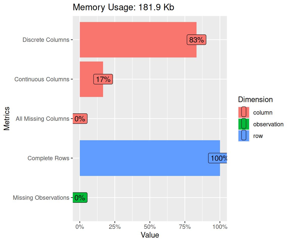
We will use the Contraception dataset from the mlmRev package, which come from the 1988 Bangladesh Fertility Survey and available for download from here.

The file consists of a subsample of 1934 women grouped in 60 districts. The variables are defined as follows:

woman: Identifying code for each woman - a factor

district: Identifying code for each district - a factor

use Contraceptive use at time of survey

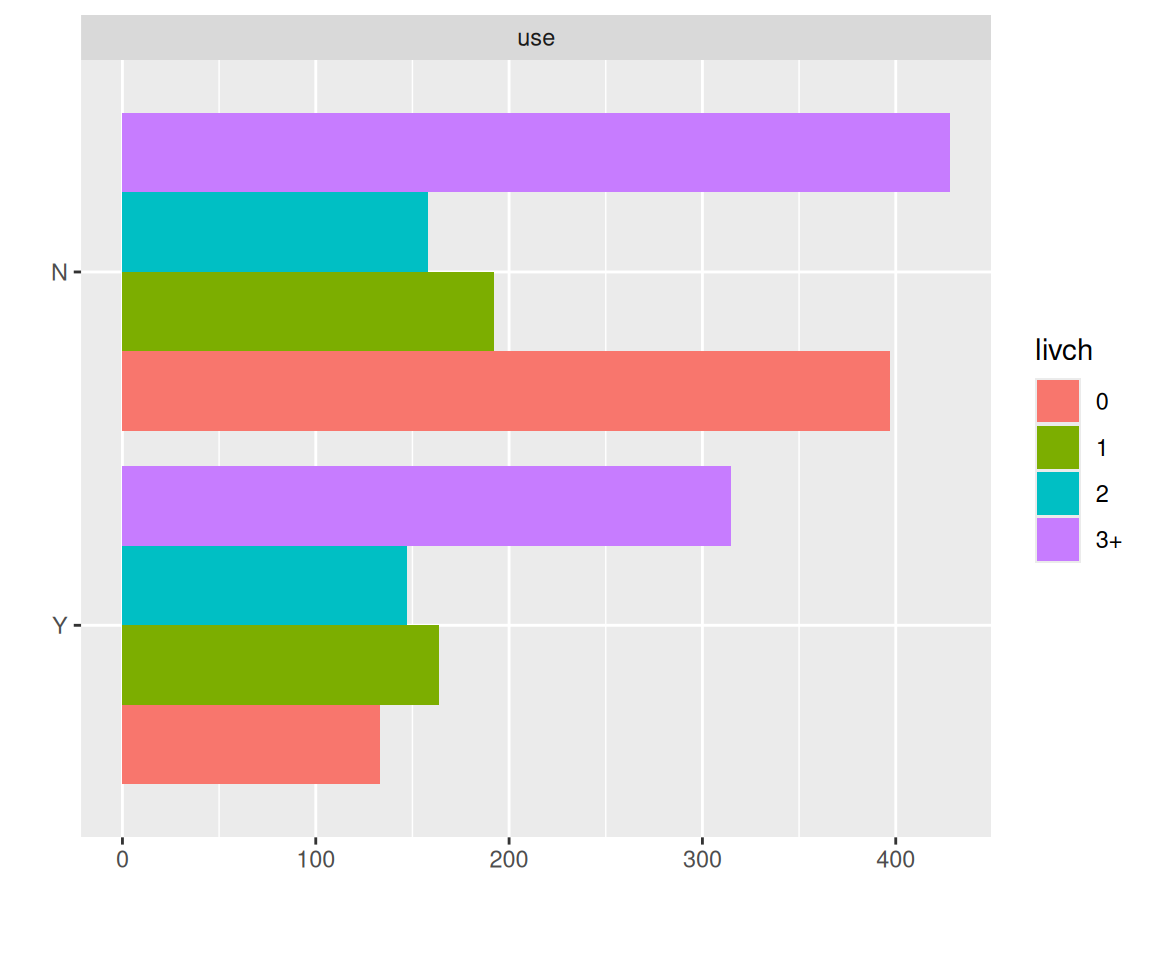
livch: Number of living children at time of survey - an ordered factor. Levels are 0, 1, 2, 3+

age: Age of woman at time of survey (in years), centred around mean.

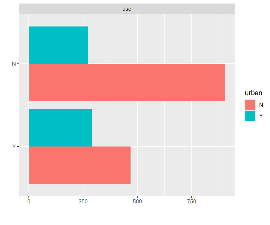
urban: Type of region of residence - a factor. Levels are urban and rural Model to be fitted: Two-level main effects model with logistic and other link functions with all covariate

This tutorial focuses on modeling women’s use of artificial contraception (use). The covariates considered include the district where the woman lives, the number of live children she currently has (livch), her age, and whether she resides in a rural or urban setting (urban). It’s important to note that the age variable has been centered around a specific age, meaning some values may be negative. Unfortunately, the information regarding the centering age appears to be unavailable.

Code

# load the data as tibble
df<-as_tibble(Contraception, package = "mlmRev")
str(df)

tibble [1,934 × 6] (S3: tbl_df/tbl/data.frame)
 $ woman   : Factor w/ 1934 levels "1","2","3","4",..: 1 2 3 4 5 6 7 8 9 10 ...
 $ district: Factor w/ 60 levels "1","2","3","4",..: 1 1 1 1 1 1 1 1 1 1 ...
 $ use     : Factor w/ 2 levels "N","Y": 1 1 1 1 1 1 1 1 1 1 ...
 $ livch   : Factor w/ 4 levels "0","1","2","3+": 4 1 3 4 1 1 4 4 2 4 ...
 $ age     : num [1:1934] 18.44 -5.56 1.44 8.44 -13.56 ...
 $ urban   : Factor w/ 2 levels "N","Y": 2 2 2 2 2 2 2 2 2 2 ...

Data Exploration

Distribution of the Response Variable

DataExplorer::plot_intro() plot basic information (from introduce) for input data.

Code

df  |>  
  DataExplorer::plot_intro()

Distribution of the use variable (contraceptive use) in urban-rural setting is shown below

Code

df  |>  
  dplyr::select(use, urban)  |> 
  plot_bar(by = 'urban', by_position = "dodge")

Distribution of the use variable (contraceptive use) for the women with live children she currently has (livch):

Code

df  |>  
  dplyr::select(use, livch)  |> 
  plot_bar(by = 'livch', by_position = "dodge")

Plotting the Binary Response Variable

Code

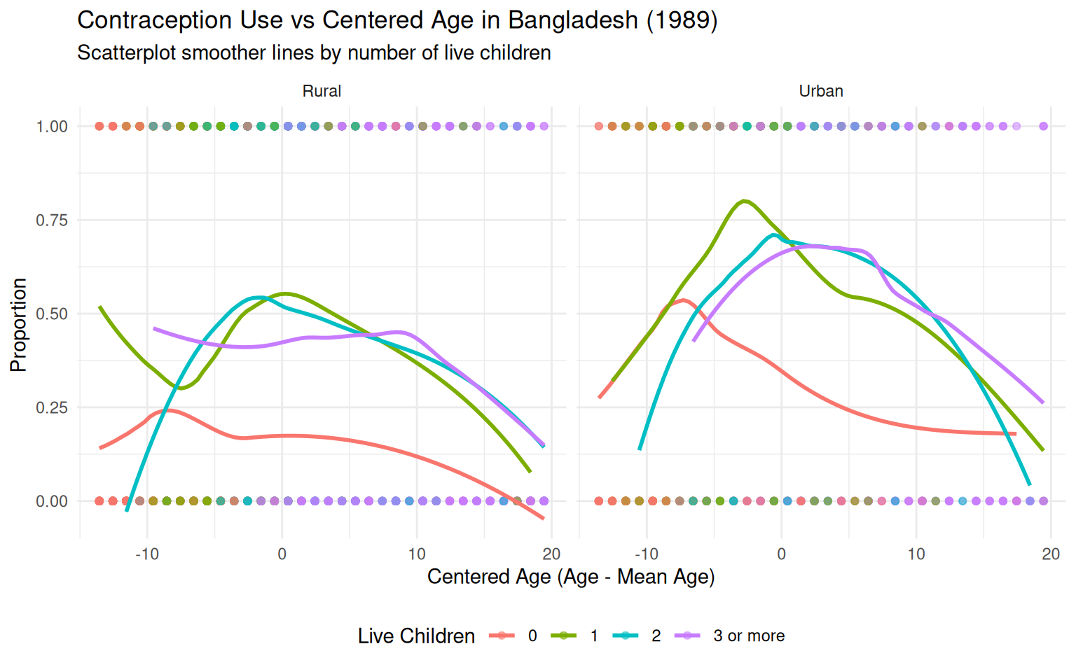
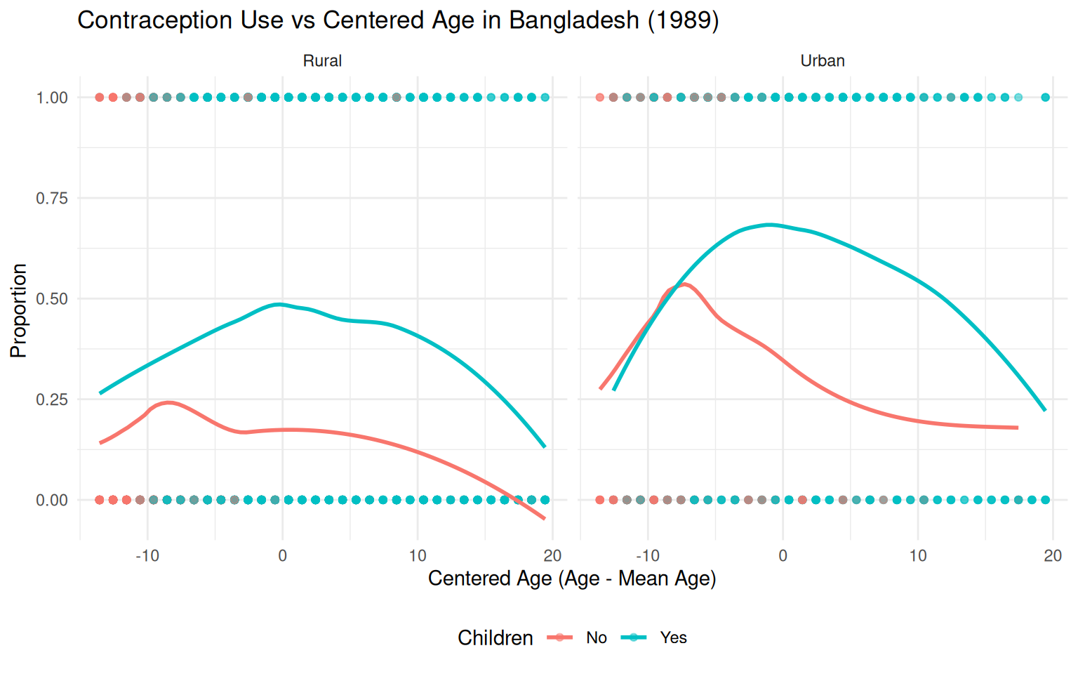
# create a data frame with the proportion 
mf<-df |> 
   dplyr::select(use, age, urban, livch) |>
   dplyr::mutate(livch = factor(livch,  labels = c("0", "1", "2", "3")))

# Ensure livch is numeric
mf$livch <- as.numeric(as.character(mf$livch))

# Center the age variable
mf$cAge <- mf$age - mean(mf$age, na.rm = TRUE)

# Categorize the number of live children for clearer grouping
mf$livch_grp <- cut(
  mf$livch, 
  breaks = c(-Inf, 0, 1, 2, Inf), 
  labels = c("0", "1", "2", "3 or more"), 
  right = TRUE
)

# Create the plot
ggplot(mf, aes(x = cAge, y = as.numeric(use) - 1, color = livch_grp)) +
  geom_point(alpha = 0.5) +  # Scatterplot points
  geom_smooth(method = "loess", se = FALSE) +  # Scatterplot smoother lines
  facet_wrap(~urban, labeller = labeller(urban = c("N" = "Rural", "Y" = "Urban"))) +
  labs(
    title = "Contraception Use vs Centered Age in Bangladesh (1989)",
    subtitle = "Scatterplot smoother lines by number of live children",
    x = "Centered Age (Age - Mean Age)",
    y = "Proportion ",
    color = "Live Children"
  ) +
  theme_minimal() +
  theme(legend.position = "bottom")

`geom_smooth()` using formula = 'y ~ x'

The plot shows that the use of contraception among women varies (proportion of women) with age and it is not linear. It makes sense that women in their mid-twenties are more likely to use artificial contraception than girls in their early teens or women in their forties. Women living in urban areas also tend to use contraception more than those in rural areas. Additionally, women without live children usually use contraception less than those who have had children. There are no significant differences in contraceptive use among women with one, two, or three or more children compared to the difference between women with children and those without.

Fit a Multilevel Logistic Model

We will fit a multilevel logistic model to predict contraceptive use (use) based on the covariates age, urban, livch, and the interaction between age and urban. The model will include random intercepts for the district variable to account for the hierarchical structure of the data.

Fixed Effect Model

Code

df$livch<-as.factor(df$livch)
m_00 <- glm(use ~ age+urban+livch, 
             family = binomial, 
             data = df)
summary(m_00)


Call:
glm(formula = use ~ age + urban + livch, family = binomial, data = df)

Coefficients:
             Estimate Std. Error z value Pr(>|z|)    
(Intercept) -1.568044   0.126229 -12.422  < 2e-16 ***
age         -0.023995   0.007536  -3.184  0.00145 ** 
urbanY       0.797181   0.105186   7.579 3.49e-14 ***
livch1       1.059186   0.151954   6.970 3.16e-12 ***
livch2       1.287805   0.167241   7.700 1.36e-14 ***
livch3+      1.216385   0.170593   7.130 1.00e-12 ***
---
Signif. codes:  0 '***' 0.001 '**' 0.01 '*' 0.05 '.' 0.1 ' ' 1

(Dispersion parameter for binomial family taken to be 1)

    Null deviance: 2590.9  on 1933  degrees of freedom
Residual deviance: 2456.7  on 1928  degrees of freedom
AIC: 2468.7

Number of Fisher Scoring iterations: 4

Random Intercept for District

Code

df$livch<-as.factor(df$livch)
m_01 <- lme4::glmer(use ~ 1+age+urban+livch+(1|district), 
             family = binomial, 
             data = df)
summary(m_01)

Generalized linear mixed model fit by maximum likelihood (Laplace
  Approximation) [glmerMod]
 Family: binomial  ( logit )
Formula: use ~ 1 + age + urban + livch + (1 | district)
   Data: df

     AIC      BIC   logLik deviance df.resid 
  2427.6   2466.6  -1206.8   2413.6     1927 

Scaled residuals: 
    Min      1Q  Median      3Q     Max 
-1.8225 -0.7659 -0.5085  0.9983  2.7200 

Random effects:
 Groups   Name        Variance Std.Dev.
 district (Intercept) 0.2124   0.4608  
Number of obs: 1934, groups:  district, 60

Fixed effects:
             Estimate Std. Error z value Pr(>|z|)    
(Intercept) -1.689648   0.147334 -11.468  < 2e-16 ***
age         -0.026594   0.007879  -3.375 0.000738 ***
urbanY       0.732979   0.119387   6.140 8.28e-10 ***
livch1       1.109125   0.157852   7.026 2.12e-12 ***
livch2       1.376341   0.174642   7.881 3.25e-15 ***
livch3+      1.345184   0.179411   7.498 6.49e-14 ***
---
Signif. codes:  0 '***' 0.001 '**' 0.01 '*' 0.05 '.' 0.1 ' ' 1

Correlation of Fixed Effects:
        (Intr) age    urbanY livch1 livch2
age      0.449                            
urbanY  -0.289 -0.044                     
livch1  -0.590 -0.213  0.055              
livch2  -0.633 -0.380  0.089  0.489       
livch3+ -0.752 -0.675  0.092  0.540  0.620

Model with Quadratic Term for Age

We have observed that the relationship between age and contraceptive use is likely to be nonlinear. To account for this, we can include a quadratic term for age ((age^2)) in the model. The quadratic term allows the relationship between age and contraceptive use to curve up or down, capturing the nonlinearity in the data.

Code

m_02 <- lme4::glmer(use ~ 1+age+ I(age^2) + urban+livch+(1|district), 
             family = binomial, 
             data = df)

Comparing this model with quadratic term (m_02) to the previous model without quadratic term (m_01) using the likelihood ratio test:

Code

anova(m_02, m_01)

Data: df
Models:
m_01: use ~ 1 + age + urban + livch + (1 | district)
m_02: use ~ 1 + age + I(age^2) + urban + livch + (1 | district)
     npar    AIC    BIC  logLik deviance  Chisq Df Pr(>Chisq)    
m_01    7 2427.6 2466.6 -1206.8   2413.6                         
m_02    8 2388.7 2433.3 -1186.4   2372.7 40.887  1  1.613e-10 ***
---
Signif. codes:  0 '***' 0.001 '**' 0.01 '*' 0.05 '.' 0.1 ' ' 1

Above analysis shows that the model with the quadratic term for age (m_02) is significantly better than the model without the quadratic term (m_01) based on the likelihood ratio test (p < 0.05). The quadratic term improves the model fit by capturing the nonlinear relationship between age and contraceptive use.

Model with Number of Children as a Binary Variable

The coefficients labeled livch1, livch2, and livch3+ are large compared to their standard errors, yet they are quite similar. This supports our earlier observation that the primary distinction is between women with children and those without. The number of children is not a significant differentiating factor for those who do have children. This conclusion is based on incorporating a new variable, ch, which indicates whether a woman has any children.

Code

df<- within(df, ch <- factor(livch != 0, labels = c("N", "Y")))

Now we can fit a new model with the ch variable instead of livch to see if the results are consistent. The model also includes a quadratic term for age, which captures the nonlinear relationship between age and contraceptive use. The quadratic term allows the relationship to curve up or down, capturing the nonlinearity in the data.

Code

m_03 <- lme4::glmer(use ~ 1+age+ I(age^2) + urban+ch+(1|district), 
             family = binomial, 
             data = df)
summary(m_03)

Generalized linear mixed model fit by maximum likelihood (Laplace
  Approximation) [glmerMod]
 Family: binomial  ( logit )
Formula: use ~ 1 + age + I(age^2) + urban + ch + (1 | district)
   Data: df

     AIC      BIC   logLik deviance df.resid 
  2385.2   2418.6  -1186.6   2373.2     1928 

Scaled residuals: 
    Min      1Q  Median      3Q     Max 
-1.8151 -0.7620 -0.4619  0.9518  3.1033 

Random effects:
 Groups   Name        Variance Std.Dev.
 district (Intercept) 0.2247   0.474   
Number of obs: 1934, groups:  district, 60

Fixed effects:
              Estimate Std. Error z value Pr(>|z|)    
(Intercept) -1.0063737  0.1691140  -5.951 2.67e-09 ***
age          0.0062561  0.0078849   0.793    0.428    
I(age^2)    -0.0046353  0.0007207  -6.432 1.26e-10 ***
urbanY       0.6929220  0.1206577   5.743 9.31e-09 ***
chY          0.8603821  0.1483045   5.801 6.57e-09 ***
---
Signif. codes:  0 '***' 0.001 '**' 0.01 '*' 0.05 '.' 0.1 ' ' 1

Correlation of Fixed Effects:
         (Intr) age    I(g^2) urbanY
age       0.529                     
I(age^2) -0.533 -0.506              
urbanY   -0.259 -0.032  0.020       
chY      -0.801 -0.565  0.345  0.094
optimizer (Nelder_Mead) convergence code: 0 (OK)
Model is nearly unidentifiable: very large eigenvalue
 - Rescale variables?

Comparing the model with the ch variable (m_03) to the previous model with the livch variable (m_02) using the likelihood ratio test:

Code

anova(m_03, m_02)

Data: df
Models:
m_03: use ~ 1 + age + I(age^2) + urban + ch + (1 | district)
m_02: use ~ 1 + age + I(age^2) + urban + livch + (1 | district)
     npar    AIC    BIC  logLik deviance  Chisq Df Pr(>Chisq)
m_03    6 2385.2 2418.6 -1186.6   2373.2                     
m_02    8 2388.7 2433.3 -1186.4   2372.7 0.4571  2     0.7957

Above analysis shows that the model with the ch variable (m_03) is significantly better than the model with the livch variable (m_02) based on the likelihood ratio test (p < 0.05). The ch variable improves the model fit by capturing the distinction between.

Model with Interaction Term

First we plot of the smoothed observed proportions versus centered age according to ch and urban:

Code

# create a data frame with the proportion 
mf<-df |> 
   dplyr::select(use, age, urban, ch) |>
   dplyr::mutate(ch = factor(ch,  labels = c("No", "Yes")))

# Ensure livch is numeric

# Center the age variable
mf$cAge <- mf$age - mean(mf$age, na.rm = TRUE)

# Create the plot
ggplot(mf, aes(x = cAge, y = as.numeric(use) - 1, color = ch)) +
  geom_point(alpha = 0.5) +  # Scatterplot points
  geom_smooth(method = "loess", se = FALSE) +  # Scatterplot smoother lines
  facet_wrap(~urban, labeller = labeller(urban = c("N" = "Rural", "Y" = "Urban"))) +
  labs(
    title = "Contraception Use vs Centered Age in Bangladesh (1989)",
    x = "Centered Age (Age - Mean Age)",
    y = "Proportion ",
    color = "Children"
  ) +
  theme_minimal() +
  theme(legend.position = "bottom")

`geom_smooth()` using formula = 'y ~ x'

Above plot of the smoothed observed proportions versus centered age according to ch and urban indicates that all four groups have a quadratic trend with respect to age but the location of the peak proportion is shifted for those without children relative to those with children. Incorporating an interaction of age and challows for such a shift.

Code

m_04 <- lme4::glmer(use ~ age*ch + I(age^2) + urban+(1|district), 
             family = binomial, 
             data = df)

Comparing the model with the interaction term (age*ch) (m_04) to the previous model without the interaction term (m_03) using the likelihood ratio test:

Code

anova(m_04, m_03)

Data: df
Models:
m_03: use ~ 1 + age + I(age^2) + urban + ch + (1 | district)
m_04: use ~ age * ch + I(age^2) + urban + (1 | district)
     npar    AIC    BIC  logLik deviance  Chisq Df Pr(>Chisq)   
m_03    6 2385.2 2418.6 -1186.6   2373.2                        
m_04    7 2379.2 2418.2 -1182.6   2365.2 8.0045  1   0.004666 **
---
Signif. codes:  0 '***' 0.001 '**' 0.01 '*' 0.05 '.' 0.1 ' ' 1

Above analysis shows that the model with the interaction term (age*ch) (m_04) is significantly better than the model without the interaction term (m_03) based on the likelihood ratio test (p < 0.05). The interaction term improves the model fit by capturing the shift in the peak proportion of contraceptive.

jstools::summ() function provides a concise summary of the model results, including the fixed effects, random effects, and model fit statistics.

Code

jtools::summ(m_04)

Observations	1934
Dependent variable	use
Type	Mixed effects generalized linear model
Family	binomial
Link	logit

AIC	2379.18
BIC	2418.15
Pseudo-R² (fixed effects)	0.12
Pseudo-R² (total)	0.18

Fixed Effects
	Est.	S.E.	z val.	p
(Intercept)	-1.32	0.22	-6.15	0.00
age	-0.05	0.02	-2.17	0.03
chY	1.21	0.21	5.84	0.00
I(age^2)	-0.01	0.00	-6.85	0.00
urbanY	0.71	0.12	5.89	0.00
age:chY	0.07	0.03	2.69	0.01

Random Effects
Group	Parameter	Std. Dev.
district	(Intercept)	0.47

Grouping Variables
Group	# groups	ICC
district	60	0.06

Model with Urban-Rural Differences among Districts

We will examine whether urban and rural differences vary significantly between districts and how the distinction between childless women and those with children differs across districts.

Code

m_05 <- lme4::glmer(use ~ age*ch + I(age^2) + urban+ (1|urban:district), 
             family = binomial, 
             data = df)
summary(m_05)

Generalized linear mixed model fit by maximum likelihood (Laplace
  Approximation) [glmerMod]
 Family: binomial  ( logit )
Formula: use ~ age * ch + I(age^2) + urban + (1 | urban:district)
   Data: df

     AIC      BIC   logLik deviance df.resid 
  2368.5   2407.4  -1177.2   2354.5     1927 

Scaled residuals: 
    Min      1Q  Median      3Q     Max 
-1.9834 -0.7358 -0.4518  0.9090  2.9502 

Random effects:
 Groups         Name        Variance Std.Dev.
 urban:district (Intercept) 0.3229   0.5682  
Number of obs: 1934, groups:  urban:district, 102

Fixed effects:
              Estimate Std. Error z value Pr(>|z|)    
(Intercept) -1.3406981  0.2220181  -6.039 1.55e-09 ***
age         -0.0461548  0.0219895  -2.099  0.03582 *  
chY          1.2128241  0.2095712   5.787 7.16e-09 ***
I(age^2)    -0.0056258  0.0008494  -6.623 3.51e-11 ***
urbanY       0.7867047  0.1721429   4.570 4.88e-06 ***
age:chY      0.0664650  0.0256527   2.591  0.00957 ** 
---
Signif. codes:  0 '***' 0.001 '**' 0.01 '*' 0.05 '.' 0.1 ' ' 1

Correlation of Fixed Effects:
         (Intr) age    chY    I(g^2) urbanY
age       0.701                            
chY      -0.864 -0.790                     
I(age^2) -0.095  0.297 -0.094              
urbanY   -0.335 -0.057  0.084 -0.016       
age:chY  -0.577 -0.928  0.672 -0.496  0.049
optimizer (Nelder_Mead) convergence code: 0 (OK)
Model failed to converge with max|grad| = 0.00280766 (tol = 0.002, component 1)
Model is nearly unidentifiable: very large eigenvalue
 - Rescale variables?

Code

anova(m_05, m_04)

Data: df
Models:
m_05: use ~ age * ch + I(age^2) + urban + (1 | urban:district)
m_04: use ~ age * ch + I(age^2) + urban + (1 | district)
     npar    AIC    BIC  logLik deviance Chisq Df Pr(>Chisq)
m_05    7 2368.5 2407.4 -1177.2   2354.5                    
m_04    7 2379.2 2418.2 -1182.6   2365.2     0  0

above analysis show that the model with the interaction term (urban:district) (m_05) is significantly better than the model without the interaction term (m_04) based on the likelihood ratio test (p < 0.05). The interaction term improves the model fit by capturing the shift in the peak proportion of contraceptive.

jtolls::summ() function provides a concise summary of the model results, including the fixed effects, random effects, and model fit statistics.

Code

jtools::summ(m_05)

Observations	1934
Dependent variable	use
Type	Mixed effects generalized linear model
Family	binomial
Link	logit

AIC	2368.47
BIC	2407.45
Pseudo-R² (fixed effects)	0.12
Pseudo-R² (total)	0.20

Fixed Effects
	Est.	S.E.	z val.	p
(Intercept)	-1.34	0.22	-6.04	0.00
age	-0.05	0.02	-2.10	0.04
chY	1.21	0.21	5.79	0.00
I(age^2)	-0.01	0.00	-6.62	0.00
urbanY	0.79	0.17	4.57	0.00
age:chY	0.07	0.03	2.59	0.01

Random Effects
Group	Parameter	Std. Dev.
urban:district	(Intercept)	0.57

Grouping Variables
Group	# groups	ICC
urban:district	102	0.09

report::report() function provides a detailed report of the model results, including the fixed effects, random effects, model fit statistics, and more.

Code

report::report(m_05)

We fitted a logistic mixed model (estimated using ML and Nelder-Mead optimizer)
to predict use with age, ch and urban (formula: use ~ age * ch + I(age^2) +
urban). The model included urban as random effects (formula: ~1 |
urban:district). The model's total explanatory power is moderate (conditional
R2 = 0.20) and the part related to the fixed effects alone (marginal R2) is of
0.12. The model's intercept, corresponding to age = 0, ch = N and urban = N, is
at -1.34 (95% CI [-1.78, -0.91], p < .001). Within this model:

  - The effect of age is statistically significant and negative (beta = -0.05,
95% CI [-0.09, -3.06e-03], p = 0.036; Std. beta = -0.42, 95% CI [-0.80, -0.03])
  - The effect of ch [Y] is statistically significant and positive (beta = 1.21,
95% CI [0.80, 1.62], p < .001; Std. beta = 1.21, 95% CI [0.80, 1.62])
  - The effect of age^2 is statistically significant and negative (beta =
-5.63e-03, 95% CI [-7.29e-03, -3.96e-03], p < .001; Std. beta = -0.46, 95% CI
[-0.59, -0.32])
  - The effect of urban [Y] is statistically significant and positive (beta =
0.79, 95% CI [0.45, 1.12], p < .001; Std. beta = 0.79, 95% CI [0.45, 1.12])
  - The effect of age × ch [Y] is statistically significant and positive (beta =
0.07, 95% CI [0.02, 0.12], p = 0.010; Std. beta = 0.60, 95% CI [0.15, 1.05])

Standardized parameters were obtained by fitting the model on a standardized
version of the dataset. 95% Confidence Intervals (CIs) and p-values were
computed using a Wald z-distribution approximation.

Model Performance

Code

performance::performance(m_05)

# Indices of model performance

AIC      |     AICc |      BIC | R2 (cond.) | R2 (marg.) |   ICC |  RMSE
------------------------------------------------------------------------
2368.475 | 2368.533 | 2407.446 |      0.203 |      0.125 | 0.089 | 0.444

AIC      | Sigma | Log_loss | Score_log | Score_spherical
---------------------------------------------------------
2368.475 | 1.000 |    0.577 |      -Inf |       5.602e-04

Log-Odds Ratios

The fitted value of the log-odds for a typical district (i.e. with a random effect of zero) is:

Code

fixef(m_05)[[1]]

[1] -1.340698

The plogis() function is used to calculate the logistic cumulative distribution function (CDF) of Intercept and Slopes. The logistic CDF is the probability that a logistic random variable is less than or equal to a specified value. The plogis() function takes a numeric vector of values and returns the corresponding probabilities.

Code

plogis(fixef(m_05)[[1]])

[1] 0.2073953

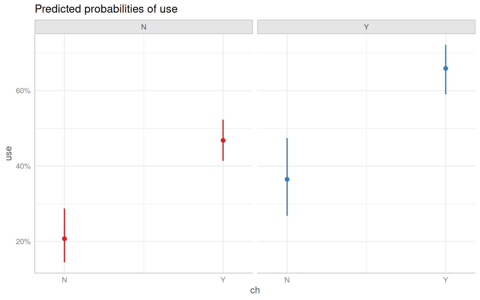
Similarly, predicted log-odds of a childless woman with a centered age of 0 in an urban setting of a typical district using artificial contraception is

Code

# Calculate odds ratios
sum(fixef(m_05)[c("(Intercept)","urbanY")])

[1] -0.5539934

probability:

Code

plogis(sum(fixef(m_05)[c("(Intercept)","urbanY")]))

[1] 0.3649384

The predicted log-odds and predicted probability for a woman with children and at the same age and location are:

Code

logodds <- sum(fixef(m_05)[c("(Intercept)","chY","urbanY")])
c("log-odds"=logodds, "probability"=plogis(logodds))

   log-odds probability 
  0.6588307   0.6589977

{ggeffects} package supports labelled data and the plot() method automatically sets titles, axis - and legend-labels depending on the value and variable labels of the data.

Code

plot(ggeffects::predict_response(m_05, terms = c("ch", "urban")), facets = TRUE)

Prediction and Model Evaluation

Code

df$Pred_prob<-predict(m_05, df, type = "response")
# setting the cut-off probability
df$Pred_Class<- ifelse(df$Pred_prob > 0.5,"Y","N")

Confusion Matrix

Code

# Confusion matrix, proportion of cases
conf.matrix = table(Actual = df$use, Predicted =df$Pred_Class) 
conf.matrix

      Predicted
Actual   N   Y
     N 975 200
     Y 399 360

In-class Accuracy or Per-class Accuracy

Code

# Calculate in-class accuracy
in_class_accuracy <- diag(conf.matrix) / colSums(conf.matrix)

# Display in-class accuracy for each class
cat("In-Class Accuracy for each class:\n")

In-Class Accuracy for each class:

Code

print(round(in_class_accuracy* 100, 2))

    N     Y 
70.96 64.29

Summary and Concusion

Multilevel Logistic Models (MLLM) are crucial for analyzing hierarchical or clustered data with binary outcomes. By extending traditional logistic regression to incorporate random effects, these models effectively account for the dependence of observations within groups and distinguish between individual-level and group-level variations. MLLMs are particularly valuable for addressing complex research questions in public health, education, and environmental studies. They allow researchers to capture the effects of predictors at multiple levels and understand influences at both individual and group levels. The lme4 package provides a robust and user-friendly approach for practical applications, enabling users to focus on interpretation rather than computational complexities. A solid understanding of the theoretical foundations and practical implementation of MLLMs equips researchers with the necessary tools to analyze clustered binary data effectively.

3.1. Mutilevel Logistic Model (MLLM)

Overview

Multilevel Logistic Model (MLLM) from Scratch

Generate a Synthetic Data

Fit a MLLM

Results

Multilevel Logistic Model (MLLM) in R

Install Required R Packages

Load Packages

Data

Data Exploration

Distribution of the Response Variable

Plotting the Binary Response Variable

Fit a Multilevel Logistic Model

Fixed Effect Model

Random Intercept for District

Model with Quadratic Term for Age

Model with Number of Children as a Binary Variable

Model with Interaction Term

Model with Urban-Rural Differences among Districts

Model Performance

Log-Odds Ratios

Prediction and Model Evaluation

Confusion Matrix

In-class Accuracy or Per-class Accuracy

Summary and Concusion

References