Asymptotic models or functions describe the behavior of functions as the input grows towards infinity or some critical point. In the context of fitting models to data, asymptotic functions often capture the concept that the response variable approaches a limiting value as the predictor variable increases. These functions are particularly useful in biological, ecological, and pharmacokinetic modeling.
Michaelis–Menten: Commonly used in biochemistry for enzyme kinetics.
2-Parameter Asymptotic Exponential: Used in modeling biological growth, decay processes, and pharmacokinetics.
3-Parameter Asymptotic Exponential: Suitable for situations where there is an initial delay before the process starts, such as latency periods in pharmacokinetics or delayed responses in ecological studies.
These models are essential tools in various scientific fields to describe processes that approach a limit but never quite reach it, providing insights into the underlying mechanisms of the observed phenomena.
Fit Asymptotic Models in R
In this tutorial, we will demonstrate how to fit asymptotic models to data using R.
Install Required R Packages
Code
# Packages Listpackages <-c("tidyverse", # Includes readr, dplyr, ggplot2, etc.'patchwork', # for visualization'minpack.lm', # for damped exponential model'nlstools', # for bootstrapping'nls2', # for fitting multiple models'broom'# for tidying model output)
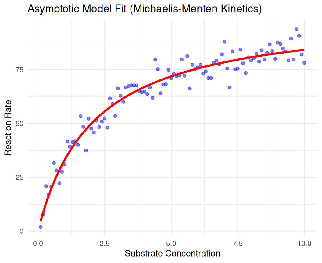
The Michaelis–Menten equation is widely used in enzyme kinetics to describe the rate of enzymatic reactions. It models how the reaction rate depends on the concentration of a substrate.
\(K_m\): Michaelis constant (substrate concentration at which the reaction rate is half of \(V_{\max}\))
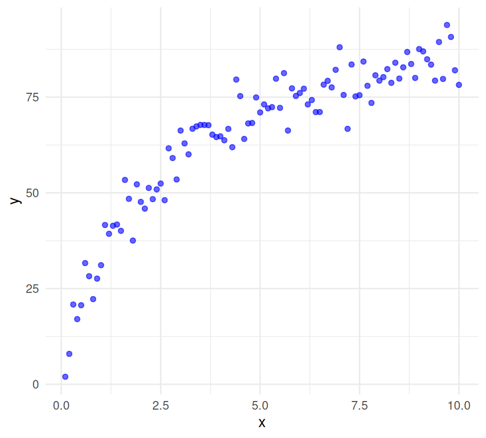
Generate Synthetic Data
Code
# Example data with noiseset.seed(123)# Generate synthetic enzyme kinetics dataset.seed(123)x<-seq(0.1, 10, length.out =100)Vmax <-100# maximum reaction rateKm <-2# Michaelis constanty <- Vmax * x / (Km + x) +rnorm(100, sd =5)# Create a data framedata.1<-data.frame(x = x, y = y)# plot dataggplot(data.1, aes(x = x, y = y)) +geom_point(alpha =0.6, color ="blue") +theme_minimal()
Code
# Define the asymptotic model function (Michaelis-Menten)asymptotic_model <-function(substrate_conc, Vmax, Km) { Vmax * substrate_conc / (Km + substrate_conc)}# Fit the asymptotic model to the data using non-linear least squaresfit.1<-nls(y ~asymptotic_model(x, Vmax, Km), data = data.1, start =list(Vmax =100, Km =2))# Get the summary of the fitsummary(fit.1)
Formula: y ~ asymptotic_model(x, Vmax, Km)

Parameters:
     Estimate Std. Error t value Pr(>|t|)
Vmax 101.6957     1.8667   54.48   <2e-16 ***
Km     2.0732     0.1279   16.21   <2e-16 ***
---
Signif. codes:  0 '***' 0.001 '**' 0.01 '*' 0.05 '.' 0.1 ' ' 1

Residual standard error: 4.578 on 98 degrees of freedom

Number of iterations to convergence: 3
Achieved convergence tolerance: 1.325e-06
# Predict using the fitted modeldata.1$pred <-predict(fit.1, newdata = data.1)# Plot the original data and the fitted asymptotic modelggplot(data.1, aes(x = x, y = y)) +geom_point(color ="blue", alpha =0.5) +geom_line(aes(y = pred), color ="red", size =1.2) +ggtitle("Asymptotic Model Fit (Michaelis-Menten Kinetics)") +xlab("Substrate Concentration") +ylab("Reaction Rate") +theme_minimal()
Warning: Using `size` aesthetic for lines was deprecated in ggplot2 3.4.0.
ℹ Please use `linewidth` instead.
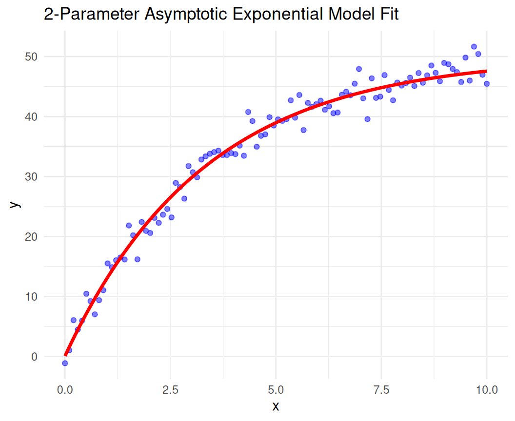
2-Parameter Asymptotic Exponential Function
This model describes a process that asymptotically approaches a maximum value with an exponential decay rate. It is often used in growth processes, pharmacokinetics, and environmental modeling.
\[ y = a \left(1 - e^{-bx}\right) \]
\(y\): Dependent variable
\(x\): Independent variable
\(a\): Asymptotic maximum value
\(b\): Rate constant
Generate Data
Code
# Generate synthetic dataset.seed(123)x <-seq(0, 10, length.out =100)asymptote <-50rate <-0.3y <- asymptote * (1-exp(-rate * x)) +rnorm(100, sd =2)# Create a data framedata.2<-data.frame(x = x, y = y)
Fit the Model
Code
# Fit the modelfit.2<-nls( y ~ asymptote + b *exp(-c * x),data = data.2,start =list(b =0.1, c =0.1) # Reasonable starting guesses)# Summary of resultssummary(fit.2)
Formula: y ~ asymptote + b * exp(-c * x)

Parameters:
    Estimate Std. Error t value Pr(>|t|)
b -49.916719   0.633496  -78.80   <2e-16 ***
c   0.301867   0.005664   53.29   <2e-16 ***
---
Signif. codes:  0 '***' 0.001 '**' 0.01 '*' 0.05 '.' 0.1 ' ' 1

Residual standard error: 1.84 on 98 degrees of freedom

Number of iterations to convergence: 11
Achieved convergence tolerance: 1.923e-07
Plot the Fitted Model
Code
# Predict using the fitted modeldata.2$pred <-predict(fit.2, newdata = data.2)# Plot the original data and the fitted asymptotic exponential modelggplot(data.2, aes(x = x, y = y)) +geom_point(color ="blue", alpha =0.5) +geom_line(aes(y = pred), color ="red", size =1.2) +ggtitle("2-Parameter Asymptotic Exponential Model Fit") +xlab("x") +ylab("y") +theme_minimal()
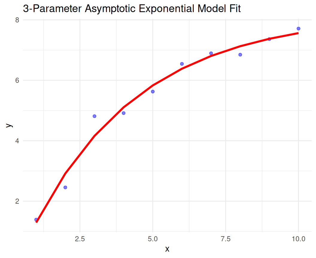
3-Parameter Asymptotic Exponential Function
This model extends the 2-parameter model by including a horizontal shift, allowing for more flexibility in fitting data where the process starts at a point other than zero.
\[ y = a \left(1 - e^{-b(x - c)}\right) \]
\(y\): Dependent variable
\(x\): Independent variable
\(a\): Asymptotic maximum value
\(b\): Rate constant
\(c\): Horizontal shift (delay before the exponential growth starts)
Data Generation
Code
# Simulating some dataset.seed(123)x <-1:10y <-c(1.5, 2.5, 4.5, 4.9, 5.6, 6.2, 6.8, 7.1, 7.5, 7.8) +rnorm(10, 0, 0.2)# Put data into a dataframedata.3<-data.frame(x, y)
Fit Using Manual Starting Values
Estimate starting values:
\(a_0\): Slightly above the maximum observed \(y\) (e.g., \(\text{max}(y) + 5\))
Linearize \(\ln(a_0 - y) = \ln(b) - c \cdot x\) to estimate \(b_0\) and \(c_0\)
Code
# Estimate starting values max_y <-max(data.3$y) a0 <- max_y +5# Adjust based on data z <-log(a0 - data.3$y) lin_model <-lm(z ~ data.3$x) b0 <-exp(coef(lin_model)[1]) c0 <--coef(lin_model)[2]# Fit the Model with `nls()`** fit.3<-nls(y ~ a - b *exp(-c * x),data = data.3,start =list(a = a0, b = b0, c = c0))summary(fit.3)
Formula: y ~ a - b * exp(-c * x)

Parameters:
  Estimate Std. Error t value Pr(>|t|)
a  8.16864    0.50583  16.149 8.49e-07 ***
b  9.00788    0.51245  17.578 4.75e-07 ***
c  0.26969    0.05218   5.169   0.0013 **
---
Signif. codes:  0 '***' 0.001 '**' 0.01 '*' 0.05 '.' 0.1 ' ' 1

Residual standard error: 0.3512 on 7 degrees of freedom

Number of iterations to convergence: 7
Achieved convergence tolerance: 7.755e-07
Plot the Fitted Model
Code
# Predict using the fitted modeldata.3$pred <-predict(fit.3, newdata = data.3)# Plot the original data and the fitted asymptotic exponential modelggplot(data.3, aes(x = x, y = y)) +geom_point(color ="blue", alpha =0.5) +geom_line(aes(y = pred), color ="red", size =1.2) +ggtitle("3-Parameter Asymptotic Exponential Model Fit") +xlab("x") +ylab("y") +theme_minimal()
Fit Asymptotic Model with Real Data
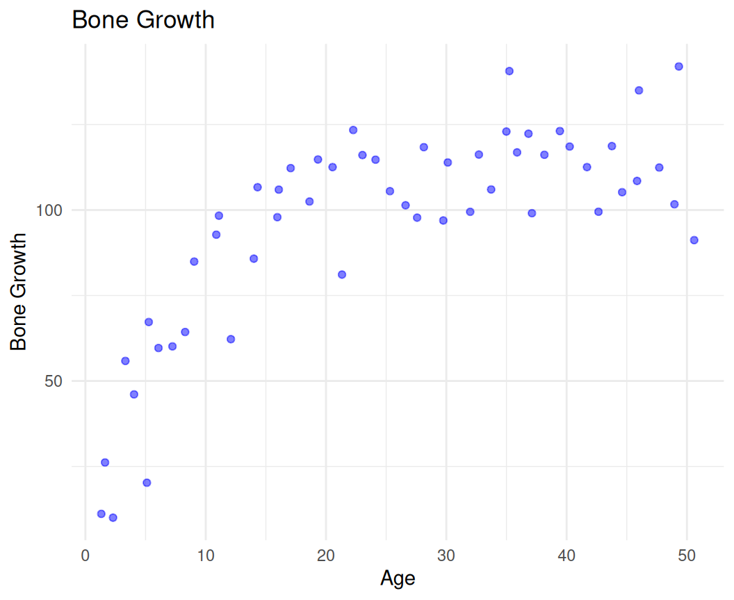
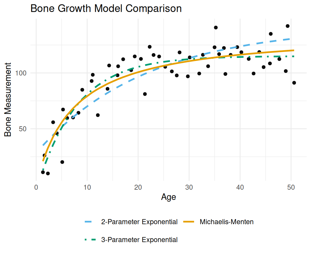
In this exercise we will fit the three models to real data on jaw growth in Deer. The data contains measurements of bone growth in rats at different ages. We will compare the performance of the Michaelis-Menten, 2-parameter asymptotic exponential, and 3-parameter asymptotic exponential models. The data is available in the file jaw_data.csv.
Code
# Load the datajaw_data <- readr::read_csv("https://github.com/zia207/r-colab/raw/main/Data/Regression_analysis/jaw_data.csv") |>filter(age >0) |># Remove age = 0glimpse()
Rows: 54 Columns: 2
── Column specification ────────────────────────────────────────────────────────
Delimiter: ","
dbl (2): age, bone

ℹ Use `spec()` to retrieve the full column specification for this data.
ℹ Specify the column types or set `show_col_types = FALSE` to quiet this message.
# Plot the original data and the fitted asymptotic exponential modelggplot(jaw_data, aes(x = age, y = bone)) +geom_point(color ="blue", alpha =0.5) +xlab("Age") +ylab("Bone Growth") +ggtitle("Bone Growth") +theme_minimal()
# Add predictionsjaw_data <- jaw_data %>%mutate(mm_pred =predict(mm_model),exp2_pred =predict(exp2_model),exp3_pred =predict(exp3_model) )# Reshape predictions into long format for legendjaw_data_long <- jaw_data %>%pivot_longer(cols =c(mm_pred, exp2_pred, exp3_pred),names_to ="Model",values_to ="Prediction" ) %>%mutate(Model =case_when( Model =="mm_pred"~"Michaelis-Menten", Model =="exp2_pred"~"2-Parameter Exponential", Model =="exp3_pred"~"3-Parameter Exponential" ) )# Define colors and linetypesmodel_colors <-c("Michaelis-Menten"="#E69F00","2-Parameter Exponential"="#56B4E9","3-Parameter Exponential"="#009E73")model_linetypes <-c("Michaelis-Menten"="solid","2-Parameter Exponential"="dashed","3-Parameter Exponential"="dotdash")ggplot(jaw_data_long, aes(x = age, y = bone)) +geom_point(alpha =0.6, color ="black") +geom_line(aes(y = Prediction, color = Model, linetype = Model),linewidth =1 ) +scale_color_manual(values = model_colors) +scale_linetype_manual(values = model_linetypes) +labs(title ="Bone Growth Model Comparison",x ="Age",y ="Bone Measurement" ) +theme_minimal() +theme(legend.position ="bottom",legend.title =element_blank(), # Remove legend titlelegend.spacing.x =unit(0.5, "cm") # Add spacing between legend items ) +guides(color =guide_legend(nrow =2), # Split color legend into 2 lineslinetype =guide_legend(nrow =2) # Split linetype legend into 2 lines )
Summary and Conclusion
In this tutorial, we explored the concept of asymptotic functions and their applications in modeling real-world phenomena using R. We specifically focused on fitting asymptotic exponential models, demonstrating how they can effectively describe processes that approach a limiting value over time.
Through nonlinear regression with nls(), we successfully estimated model parameters and visualized the fitted function, emphasizing the importance of selecting appropriate starting values for convergence. Additionally, we discussed model evaluation techniques, including residual analysis, to assess goodness-of-fit.
Understanding asymptotic functions is crucial in various fields such as biology, economics, and engineering, where growth, decay, or saturation processes are prevalent. Mastering these techniques in R allows for more accurate predictions and deeper insights into data behavior.
References
Books on Asymptotic Functions & Nonlinear Modeling
“Asymptotic Expansions and Asymptotic Distributions” – Norman Bleistein & Richard A. Handelsman
Covers asymptotic analysis techniques with practical applications in mathematical modeling.
“Mathematical Analysis: A Modern Approach to Advanced Calculus” – Tom M. Apostol
Discusses asymptotic functions in the context of advanced calculus and real analysis.
“Nonlinear Regression with R” – Christian Ritz & Jens C. Streibig
A practical guide on nonlinear regression, including asymptotic function fitting using R.
“Introduction to Asymptotics and Special Functions” – F.W.J. Olver
A foundational book covering asymptotic expansions, special functions, and their applications.
“Nonlinear Time Series: Nonparametric and Parametric Methods” – Jianqing Fan & Qiwei Yao
Covers nonlinear modeling techniques relevant to time series and asymptotic behaviors.