3.4. Mutilevel or Mixed Effect Poisson Model (MLPM)

Multi-level count data is commonly found in ecology, epidemiology, and social sciences, representing occurrences like disease cases or animal sightings. When this data is clustered or hierarchical, mixed-effects Poisson models offer a robust analytical framework. This tutorial provides an overview of mixed-effects Poisson models for count data and step-by-step instructions for fitting these models in R, highlighting the underlying principles. We will also explore several R packages, including {lme4}, {glmmTMB}, and {MASS}, to fit various Poisson models, with a particular emphasis on managing overdispersion using quasi-Poisson and negative binomial models. By the end of this tutorial, readers will gain theoretical knowledge and practical skills to analyze count data effectively, enabling informed, data-driven decision-making.

Overview

A mixed-effects Poisson model is a type of regression model used to analyze count data while accounting for both fixed effects (effects that are constant across observations) and random effects (effects that vary across groups or clusters). This model is widely used in fields such as biostatistics, epidemiology, and ecology to analyze data with hierarchical or clustered structures.

Model Description:

The general form of a mixed-effects Poisson model can be written as:

\[ Y_{ij} \sim \text{Poisson}(\lambda_{ij}) \] where:

$Y_{ij}$ is the observed count for the $i$-th observation in the $j$-th group.
$\lambda_{ij}$ is the expected count (mean) for the $i$-th observation in the $j$-th group.

The expected count, $\lambda_{ij}$, is linked to a linear predictor via a log-link function:

\[ \log(\lambda_{ij}) = X_{ij}^T \beta + Z_j^T u_j \] where:

$X_{ij}$ is a vector of fixed-effect covariates for the $i$-th observation in the $j$-th group.
$\beta$ is the vector of fixed-effect coefficients (parameters).
$Z_j$ is a vector of random-effect covariates associated with the $j$-th group.
$u_j$ is the random-effect vector for the $j$-th group, typically assumed to follow a multivariate normal distribution: $u_j \sim N(0, \Sigma_u)$.

Key Components:

Fixed Effects ($X_{ij}^T \beta$):
- Represent the population-level effects that are consistent across all groups.
- For example, the effect of a treatment or other covariates like age or gender.
Random Effects ($Z_j^T u_j$):
- Capture the group-specific variability.
- Allow for the inclusion of cluster-level heterogeneity.
Poisson Assumption:
- The response variable $Y_{ij}$ is assumed to follow a Poisson distribution with mean $\lambda_{ij}$.
- Variance equals the mean in a standard Poisson model, but overdispersion (variance greater than the mean) can be handled by extending the model (e.g., using a negative binomial distribution).

Complete Model Equation:

\[ \log(\lambda_{ij}) = \beta_0 + \sum_{k=1}^p \beta_k X_{ijk} + \sum_{m=1}^q u_{jm} Z_{ijm} \]

where:

$\beta_0$ is the intercept.
$\beta_k$ are fixed-effect coefficients for covariates $X_{ijk}$.
$u_{jm}$ are random effects for covariates (Z_{ijm}).

Variance-Covariance Structure

The random effects, (u_j), are assumed to follow a multivariate normal distribution:

\[ u_j \sim N(0, \Sigma_u) \]

where $\Sigma_u$ is the variance-covariance matrix that describes the structure of the random effects.

Inference and Estimation:

Parameters $$ (fixed effects) and $\Sigma_u$ (random effects variance-covariance) are typically estimated using maximum likelihood estimation (MLE) or Bayesian methods.
Numerical techniques like Laplace approximation or Gauss-Hermite quadrature are often used due to the complexity of the likelihood function.

Multilevel Poisson Model from Scratch

Fitting a multilevel Poisson model from scratch in R without relying on any specific packages is a computationally intensive task, as it requires implementing iterative optimization for the likelihood function. Below is a step-by-step implementation outline:

Simulated Hierarchical Data: Simulate or provide hierarchical count data with fixed and random effects.
Model Specification: Specify the likelihood function for a Poisson distribution with both fixed and random effects.
Optimization: Use numerical methods like gradient descent or Newton-Raphson to optimize the parameters.
Estimation of Random Effects: Use an iterative approach to account for random effects (e.g., via the expectation-maximization (EM) algorithm).

Simulated Hierarchical Data

Let’s start by simulating hierarchical count data with fixed and random effects. We will generate a dataset with multiple groups, each containing observations with a Poisson-distributed response variable. The data will include a covariate (e.g., age) and group-level random effects.

Code

# Step 1: Simulate Example Data
set.seed(123)

# Number of groups and observations per group
n_groups <- 10
n_obs_per_group <- 50

# Fixed effect parameters
beta_0 <- 1.5  # Intercept
beta_1 <- 0.3  # Slope for fixed effect (e.g., covariate effect)

# Random effect standard deviation
sigma_u <- 0.5  

# Generate group-level random effects
group_ids <- rep(1:n_groups, each = n_obs_per_group)
u <- rnorm(n_groups, mean = 0, sd = sigma_u)

# Covariate (e.g., age)
x <- runif(n_groups * n_obs_per_group, 0, 10)

# Generate response variable (Poisson counts)
lambda <- exp(beta_0 + beta_1 * x + u[group_ids])
y <- rpois(n_groups * n_obs_per_group, lambda)

# Data frame
data <- data.frame(group = group_ids, x = x, y = y)
head(data)

  group        x  y
1     1 8.895393 45
2     1 6.928034 17
3     1 6.405068 29
4     1 9.942698 85
5     1 6.557058 31
6     1 7.085305 27

Log-Likelihood Function

Next, we define the log-likelihood function for the mixed-effects Poisson model. The function takes the model parameters (fixed effects, random effects, and variance of random effects) as input and returns the negative log-likelihood value to be minimized during optimization. The log-likelihood consists of two components: the Poisson log-likelihood for the response variable and the log-likelihood for the random effects (prior distribution). The random effects are assumed to follow a normal distribution with mean 0 and variance $\sigma_u^2$. The total log-likelihood is the sum of these two components.

Code

# Step 2: Log-Likelihood Function
log_likelihood <- function(params) {
  beta_0 <- params[1]  # Intercept (fixed effect)
  beta_1 <- params[2]  # Covariate effect (fixed effect)
  sigma_u <- exp(params[3])  # Variance of random effects (positive)
  
  # Extract group-level random effects
  u <- params[4:(3 + n_groups)]
  
  # Calculate linear predictor
  eta <- beta_0 + beta_1 * data$x + u[data$group]
  
  # Poisson log-likelihood
  ll <- sum(data$y * eta - exp(eta))
  
  # Random effect log-likelihood (prior)
  ll_random <- sum(dnorm(u, mean = 0, sd = sigma_u, log = TRUE))
  
  # Total log-likelihood
  return(-(ll + ll_random))  # Return negative for minimization
}

Optimize Parameters using `optim()` and fit the model

We use the optim() function to optimize the log-likelihood function and estimate the fixed and random effects parameters. The initial values for the parameters are set based on prior knowledge or random values. The optimization method (e.g., BFGS) and control parameters (e.g., maximum iterations) can be specified to fine-tune the optimization process.

Code

# Step 3: Optimize Parameters
# Initial values: intercept, slope, log(sigma_u), random effects
init_params <- c(1, 0.1, log(0.5), rep(0, n_groups))

# Optimize using optim
fit <- optim(
  par = init_params,
  fn = log_likelihood,
  method = "BFGS",
  control = list(maxit = 1000)
)

Extract Results

Finally, we extract the estimated fixed effects, random effects, and variance of random effects from the optimization results. These estimates provide insights into the relationships between the covariates and the response variable, as well as the variability across groups.

Code

# Step 4: Extract Results
# Fixed effects
beta_0_est <- fit$par[1]
beta_1_est <- fit$par[2]

# Random effects
sigma_u_est <- exp(fit$par[3])
u_est <- fit$par[4:(3 + n_groups)]

# Print results
cat("Estimated Fixed Effects:\n")

Estimated Fixed Effects:

Code

cat("  Intercept (beta_0):", beta_0_est, "\n")

  Intercept (beta_0): 1.483758

Code

cat("  Slope (beta_1):", beta_1_est, "\n")

  Slope (beta_1): 0.306567

Code

cat("\nEstimated Random Effect Variance:\n")


Estimated Random Effect Variance:

Code

cat("  sigma_u:", sigma_u_est, "\n")

  sigma_u: 0.4543848

Code

cat("\nEstimated Random Effects:\n")


Estimated Random Effects:

Code

print(u_est)

 [1] -0.30456806 -0.15772944  0.74870962 -0.02052520  0.03539855  0.81127347
 [7]  0.21466981 -0.68227191 -0.40154883 -0.24085780

Multilevel Poisson Model in R

Multilevel Poisson models can be fitted using various R packages that provide robust and efficient implementations for analyzing hierarchical count data. In this section, we will demonstrate how to fit mixed-effects Poisson models using the {lme4}, {glmmTMB}, and {MASS} packages in R, highlighting the key steps involved in the modeling process.

Install Required R Packages

Following R packages are required to run this notebook. If any of these packages are not installed, you can install them using the code below:

Code

packages <- c('tidyverse',
              'dlookr',
              'sjPlot',
              'jtools',
              'lme4',
              'glmmTMB',
              'MASS',
              'MuMIn',
              'performance',
              'vcd'
         )

#| warning: false
#| error: false

# Install missing packages
new_packages <- packages[!(packages %in% installed.packages()[,"Package"])]
if(length(new_packages)) install.packages(new_packages)

# Verify installation
cat("Installed packages:\n")
print(sapply(packages, requireNamespace, quietly = TRUE))

Load Packages

Code

# Load packages with suppressed messages
invisible(lapply(packages, function(pkg) {
  suppressPackageStartupMessages(library(pkg, character.only = TRUE))
}))

Code

# Check loaded packages
cat("Successfully loaded packages:\n")

Successfully loaded packages:

Code

print(search()[grepl("package:", search())])

 [1] "package:vcd"         "package:grid"        "package:performance"
 [4] "package:MuMIn"       "package:MASS"        "package:glmmTMB"    
 [7] "package:lme4"        "package:Matrix"      "package:jtools"     
[10] "package:sjPlot"      "package:dlookr"      "package:lubridate"  
[13] "package:forcats"     "package:stringr"     "package:dplyr"      
[16] "package:purrr"       "package:readr"       "package:tidyr"      
[19] "package:tibble"      "package:ggplot2"     "package:tidyverse"  
[22] "package:stats"       "package:graphics"    "package:grDevices"  
[25] "package:utils"       "package:datasets"    "package:methods"    
[28] "package:base"

Data

In this section we use the Salamanders data set from the {glmmTMB} package. The data set containing counts of salamanders with site covariates and sampling covariates. Each of 23 sites was sampled 4 times. (Price et al. (2016); Price et al. 2015).

A data frame with 644 observations on the following 10 variables:

site: name of a location where repeated samples were taken

mined: factor indicating whether the site was affected by mountain top removal coal mining

cover: amount of cover objects in the stream (scaled)

sample: repeated sample

DOP:Days since precipitation (scaled)

Wtemp:water temperature (scaled)

DOY:day of year (scaled)

spp:abbreviated species name, possibly also life stage

count:number of salamanders observed

Price SJ, Muncy BL, Bonner SJ, Drayer AN, Barton CD (2016) Effects of mountaintop removal mining and valley filling on the occupancy and abundance of stream salamanders. Journal of Applied Ecology 53 459–468. doi:10.1111/1365-2664.12585

Price SJ, Muncy BL, Bonner SJ, Drayer AN, Barton CD (2015) Data from: Effects of mountaintop removal mining and valley filling on the occupancy and abundance of stream salamanders. Dryad Digital Repository. doi:10.5061/dryad.5m8f6

Code

mf<-as_tibble(Salamanders, package = "glmmTMB")
str(mf)

tibble [644 × 9] (S3: tbl_df/tbl/data.frame)
 $ site  : Ord.factor w/ 23 levels "R-1"<"R-2"<"R-3"<..: 13 14 15 1 2 3 4 5 6 7 ...
 $ mined : Factor w/ 2 levels "yes","no": 1 1 1 2 2 2 2 2 2 2 ...
 $ cover : num [1:644] -1.442 0.298 0.398 -0.448 0.597 ...
 $ sample: int [1:644] 1 1 1 1 1 1 1 1 1 1 ...
 $ DOP   : num [1:644] -0.596 -0.596 -1.191 0 0.596 ...
 $ Wtemp : num [1:644] -1.2294 0.0848 1.0142 -3.0234 -0.1443 ...
 $ DOY   : num [1:644] -1.497 -1.497 -1.294 -2.712 -0.687 ...
 $ spp   : Factor w/ 7 levels "GP","PR","DM",..: 1 1 1 1 1 1 1 1 1 1 ...
 $ count : int [1:644] 0 0 0 2 2 1 1 2 4 1 ...

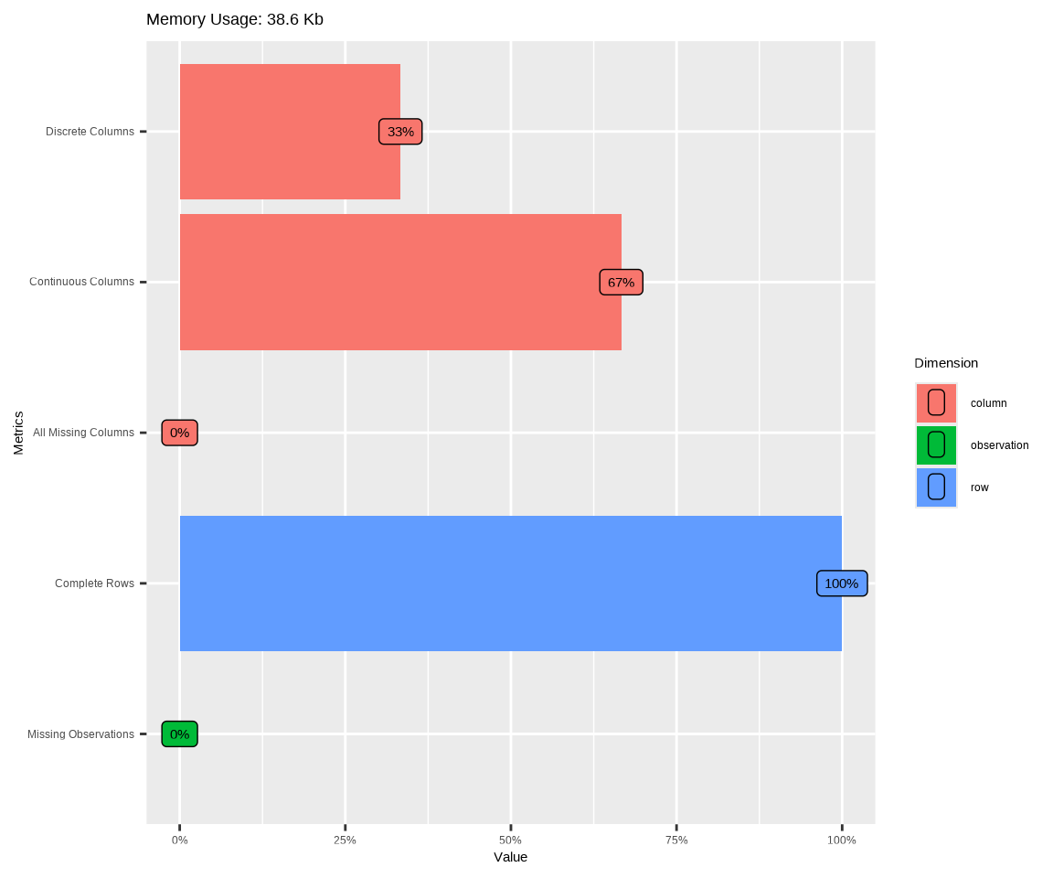
DataExplorer::plot_intro() plot basic information (from introduce) for input data.

Code

mf  |>  
  DataExplorer::plot_intro()

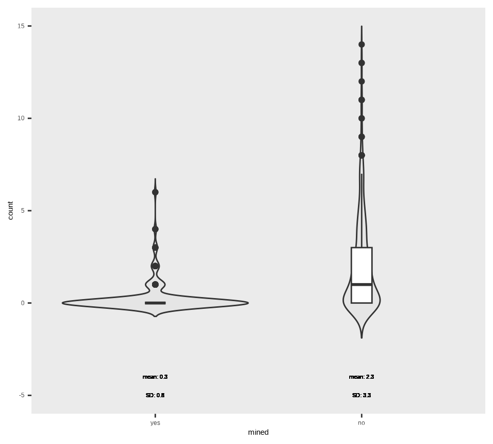
Distribution of the count variable in mined setting is shown below

Code

# output the results
mf %>%
  # prepare data
  dplyr::select(mined, count) %>%
  dplyr::group_by(mined) %>%
  dplyr::mutate(Mean = round(mean(count), 1)) %>%
  dplyr::mutate(SD = round(sd(count), 1)) %>%
  # start plot
  ggplot(aes(mined, count, color = mined, fill = mined)) +
  geom_violin(trim=FALSE, color = "gray20")+ 
  geom_boxplot(width=0.1, fill="white", color = "gray20") +
  geom_text(aes(y=-4,label=paste("mean: ", Mean, sep = "")), size = 3, color = "black") +
  geom_text(aes(y=-5,label=paste("SD: ", SD, sep = "")), size = 3, color = "black") +
  scale_fill_manual(values=rep("grey90",4)) + 
  theme_set(theme_bw(base_size = 10)) +
  theme(legend.position="none", legend.title = element_blank(),
        panel.grid.major = element_blank(),
        panel.grid.minor = element_blank()) + 
  ylim(-5, 15) +
  labs(x = "mined", y = "count")

Goodness-of-fit Tests

Code

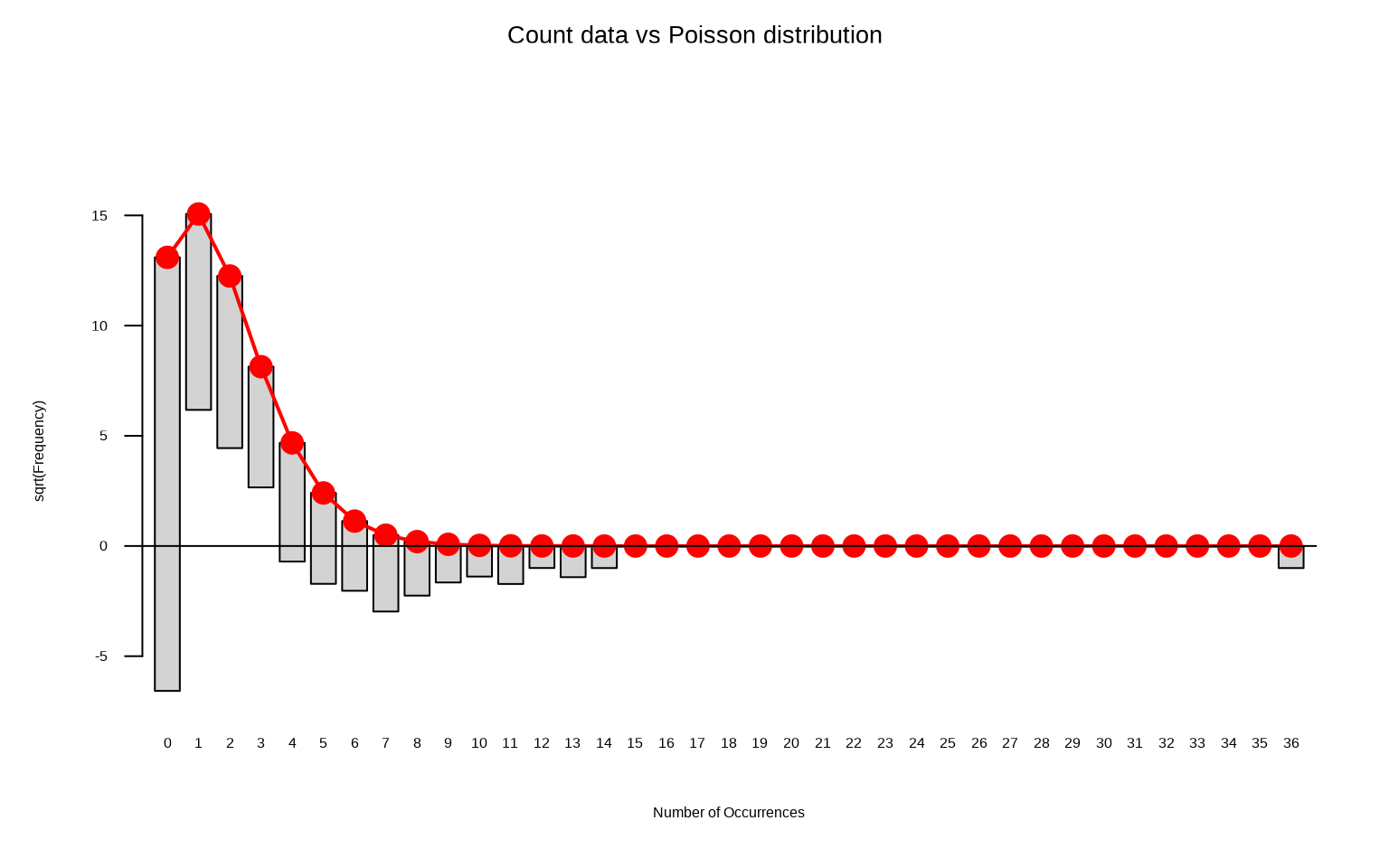
gf = vcd::goodfit(mf$count,type= "poisson", method= "ML")
plot(gf, main="Count data vs Poisson distribution")

The data does not perfectly match a Poisson distribution. We will use a goodness-of-fit test to determine if it significantly diverges from this distribution. A p-value less than .05 indicates a significant difference, suggesting the data is likely over-dispersed.

Code

summary(gf)


     Goodness-of-fit test for poisson distribution

                      X^2 df      P(> X^2)
Likelihood Ratio 958.8815 14 1.032889e-195

The p-value is indeed smaller than .05 which means that we should indeed use a negative-binomial model rather than a Poisson model. We will ignore this, for now, and proceed to fit a Poisson mixed-effects model and check what happens if a Poisson model is fit to over-dispersed data.

Mixed Effect Poisson Models

To analyze the Salamanders dataset from the {glmmTMB} package using different types of Poisson models with the {lme4} package, you can follow these steps. Here’s a detailed approach to fit fixed-effects, random-effects, and nested random-effects Poisson models.

We will fit the following models to the Salamanders dataset to model the count of salamanders observed using the cover, mined and spp variables:

Fixed-Effects Poisson Model

This model assumes only fixed effects without any grouping structure.

Code

# Fixed-effects Poisson model
model_fixed <- glm(count ~ mined + spp + cover, data = mf, family = "poisson")
summary(model_fixed)


Call:
glm(formula = count ~ mined + spp + cover, family = "poisson", 
    data = mf)

Coefficients:
            Estimate Std. Error z value Pr(>|z|)    
(Intercept) -1.49204    0.14129 -10.560  < 2e-16 ***
minedno      2.29902    0.12005  19.151  < 2e-16 ***
sppPR       -1.38629    0.21517  -6.443 1.17e-10 ***
sppDM        0.23052    0.12889   1.789   0.0737 .  
sppEC-A     -0.77011    0.17105  -4.502 6.73e-06 ***
sppEC-L      0.62117    0.11931   5.206 1.92e-07 ***
sppDES-L     0.67916    0.11813   5.749 8.96e-09 ***
sppDF        0.08004    0.13344   0.600   0.5486    
cover       -0.23087    0.04136  -5.582 2.37e-08 ***
---
Signif. codes:  0 '***' 0.001 '**' 0.01 '*' 0.05 '.' 0.1 ' ' 1

(Dispersion parameter for poisson family taken to be 1)

    Null deviance: 2120.7  on 643  degrees of freedom
Residual deviance: 1278.9  on 635  degrees of freedom
AIC: 2020.1

Number of Fisher Scoring iterations: 6

Random-Intercept Model

This model includes a random intercept for the site.

Code

# Random-intercept Poisson model
model_random_intercept <- glmer(count ~ mined + spp + cover + (1 | site), 
                                data = Salamanders, family = "poisson")
summary(model_random_intercept)

Generalized linear mixed model fit by maximum likelihood (Laplace
  Approximation) [glmerMod]
 Family: poisson  ( log )
Formula: count ~ mined + spp + cover + (1 | site)
   Data: Salamanders

     AIC      BIC   logLik deviance df.resid 
  1964.3   2009.0   -972.1   1944.3      634 

Scaled residuals: 
    Min      1Q  Median      3Q     Max 
-2.6063 -0.7421 -0.4244  0.0778 11.6872 

Random effects:
 Groups Name        Variance Std.Dev.
 site   (Intercept) 0.3175   0.5635  
Number of obs: 644, groups:  site, 23

Fixed effects:
            Estimate Std. Error z value Pr(>|z|)    
(Intercept) -1.68944    0.25581  -6.604 4.00e-11 ***
minedno      2.39498    0.33283   7.196 6.21e-13 ***
sppPR       -1.38629    0.21417  -6.473 9.63e-11 ***
sppDM        0.23050    0.12830   1.797   0.0724 .  
sppEC-A     -0.77013    0.17027  -4.523 6.10e-06 ***
sppEC-L      0.62115    0.11876   5.230 1.69e-07 ***
sppDES-L     0.67914    0.11758   5.776 7.66e-09 ***
sppDF        0.08004    0.13283   0.603   0.5468    
cover       -0.12046    0.16414  -0.734   0.4630    
---
Signif. codes:  0 '***' 0.001 '**' 0.01 '*' 0.05 '.' 0.1 ' ' 1

Correlation of Fixed Effects:
         (Intr) minedn sppPR  sppDM  spEC-A spEC-L sDES-L sppDF 
minedno  -0.777                                                 
sppPR    -0.167  0.000                                          
sppDM    -0.280  0.000  0.334                                   
sppEC-A  -0.211  0.000  0.252  0.420                            
sppEC-L  -0.302  0.000  0.361  0.602  0.454                     
sppDES-L -0.305  0.000  0.364  0.608  0.458  0.657              
sppDF    -0.270  0.000  0.322  0.538  0.406  0.582  0.587       
cover     0.385 -0.565  0.000  0.000  0.000  0.000  0.000  0.000

Random-Intercept and Slope Model

This model includes a random slope for mined within site.

Code

# Random-intercept and slope Poisson model
model_random_slope <- glmer(count ~ mined + spp + cover + (mined | site), 
                            data = mf, family = "poisson")
summary(model_random_slope)

Generalized linear mixed model fit by maximum likelihood (Laplace
  Approximation) [glmerMod]
 Family: poisson  ( log )
Formula: count ~ mined + spp + cover + (mined | site)
   Data: mf

     AIC      BIC   logLik deviance df.resid 
  1951.4   2005.0   -963.7   1927.4      632 

Scaled residuals: 
    Min      1Q  Median      3Q     Max 
-2.5719 -0.7403 -0.3875  0.0571 11.9113 

Random effects:
 Groups Name        Variance Std.Dev. Corr 
 site   (Intercept) 1.170    1.082         
        minedno     1.411    1.188    -0.99
Number of obs: 644, groups:  site, 23

Fixed effects:
            Estimate Std. Error z value Pr(>|z|)    
(Intercept) -1.98239    0.38025  -5.213 1.85e-07 ***
minedno      2.78291    0.38356   7.255 4.00e-13 ***
sppPR       -1.38764    0.21434  -6.474 9.54e-11 ***
sppDM        0.22983    0.12834   1.791 0.073337 .  
sppEC-A     -0.77091    0.17035  -4.525 6.03e-06 ***
sppEC-L      0.62020    0.11880   5.220 1.79e-07 ***
sppDES-L     0.67823    0.11763   5.766 8.12e-09 ***
sppDF        0.07872    0.13290   0.592 0.553623    
cover       -0.26668    0.07922  -3.366 0.000762 ***
---
Signif. codes:  0 '***' 0.001 '**' 0.01 '*' 0.05 '.' 0.1 ' ' 1

Correlation of Fixed Effects:
         (Intr) minedn sppPR  sppDM  spEC-A spEC-L sDES-L sppDF 
minedno  -0.951                                                 
sppPR    -0.113  0.000                                          
sppDM    -0.188  0.000  0.334                                   
sppEC-A  -0.142  0.000  0.251  0.420                            
sppEC-L  -0.203  0.000  0.360  0.602  0.454                     
sppDES-L -0.205  0.000  0.364  0.608  0.458  0.657              
sppDF    -0.182  0.000  0.322  0.538  0.405  0.581  0.587       
cover     0.144 -0.247  0.000  0.000  0.000  0.000  0.000  0.000
optimizer (Nelder_Mead) convergence code: 0 (OK)
unable to evaluate scaled gradient
Model failed to converge: degenerate  Hessian with 1 negative eigenvalues

Nested Random-Effects Model

This model includes spp nested within site.

Code

# Nested random-effects Poisson model
model_nested <- glmer(count ~ mined + cover+ spp+ (1 | site / spp), 
                      data = mf, family = "poisson")
summary(model_nested)

Generalized linear mixed model fit by maximum likelihood (Laplace
  Approximation) [glmerMod]
 Family: poisson  ( log )
Formula: count ~ mined + cover + spp + (1 | site/spp)
   Data: mf

     AIC      BIC   logLik deviance df.resid 
  1771.2   1820.4   -874.6   1749.2      633 

Scaled residuals: 
    Min      1Q  Median      3Q     Max 
-2.2697 -0.6227 -0.3389  0.0853  5.8701 

Random effects:
 Groups   Name        Variance Std.Dev.
 spp:site (Intercept) 0.7380   0.8591  
 site     (Intercept) 0.2582   0.5081  
Number of obs: 644, groups:  spp:site, 161; site, 23

Fixed effects:
            Estimate Std. Error z value Pr(>|z|)    
(Intercept) -2.15026    0.36033  -5.967 2.41e-09 ***
minedno      2.47549    0.36686   6.748 1.50e-11 ***
cover       -0.06995    0.17936  -0.390 0.696525    
sppPR       -1.35817    0.39416  -3.446 0.000569 ***
sppDM        0.42274    0.33186   1.274 0.202714    
sppEC-A     -0.61106    0.35810  -1.706 0.087931 .  
sppEC-L      0.54770    0.33040   1.658 0.097384 .  
sppDES-L     0.83687    0.32505   2.575 0.010036 *  
sppDF        0.34575    0.33353   1.037 0.299903    
---
Signif. codes:  0 '***' 0.001 '**' 0.01 '*' 0.05 '.' 0.1 ' ' 1

Correlation of Fixed Effects:
         (Intr) minedn cover  sppPR  sppDM  spEC-A spEC-L sDES-L
minedno  -0.647                                                 
cover     0.282 -0.552                                          
sppPR    -0.383 -0.027  0.018                                   
sppDM    -0.527  0.042 -0.005  0.440                            
sppEC-A  -0.455  0.000  0.001  0.410  0.491                     
sppEC-L  -0.515  0.025  0.017  0.443  0.533  0.491              
sppDES-L -0.538  0.040  0.009  0.450  0.545  0.501  0.545       
sppDF    -0.532  0.045  0.007  0.439  0.533  0.489  0.533  0.545
optimizer (Nelder_Mead) convergence code: 0 (OK)
Model failed to converge with max|grad| = 0.0140583 (tol = 0.002, component 1)

Compare Models

Now we compare the models with AIC to determine the best-fitting model.

Code

AIC(model_fixed, model_random_intercept, model_random_slope, model_nested)

                       df      AIC
model_fixed             9 2020.132
model_random_intercept 10 1964.282
model_random_slope     12 1951.433
model_nested           11 1771.211

We can also use the anova() function to compare the models using a likelihood ratio test.

Code

anova(model_fixed, model_random_intercept, model_random_slope, model_nested)

Analysis of Deviance Table

Model: poisson, link: log

Response: count

Terms added sequentially (first to last)

      Df Deviance Resid. Df Resid. Dev  Pr(>Chi)    
NULL                    643     2120.7              
mined  1   545.44       642     1575.2 < 2.2e-16 ***
spp    6   264.89       636     1310.3 < 2.2e-16 ***
cover  1    31.47       635     1278.9 2.023e-08 ***
---
Signif. codes:  0 '***' 0.001 '**' 0.01 '*' 0.05 '.' 0.1 ' ' 1

Nexted model is the best fit model based on AIC and likelihood ratio test.

Model Summary

jtolls::summ() function provides a concise summary of the model results, including the fixed effects, random effects, and model fit statistics.

Code

jtools::summ(model_nested)

Observations	644
Dependent variable	count
Type	Mixed effects generalized linear model
Family	poisson
Link	log

AIC	1771.21
BIC	1820.36
Pseudo-R² (fixed effects)	0.46
Pseudo-R² (total)	0.70

Fixed Effects
	Est.	S.E.	z val.	p
(Intercept)	-2.15	0.36	-5.97	0.00
minedno	2.48	0.37	6.75	0.00
cover	-0.07	0.18	-0.39	0.70
sppPR	-1.36	0.39	-3.45	0.00
sppDM	0.42	0.33	1.27	0.20
sppEC-A	-0.61	0.36	-1.71	0.09
sppEC-L	0.55	0.33	1.66	0.10
sppDES-L	0.84	0.33	2.57	0.01
sppDF	0.35	0.33	1.04	0.30

Random Effects
Group	Parameter	Std. Dev.
spp:site	(Intercept)	0.86
site	(Intercept)	0.51

Grouping Variables
Group	# groups	ICC
spp:site	161	0.37
site	23	0.13

Model Performance

performance::performance() function provides a summary of the model performance, including the AIC, BIC, and other fit statistics.

Code

performance::performance(model_nested)

# Indices of model performance

AIC      |     AICc |      BIC | R2 (cond.) | R2 (marg.) |   ICC |  RMSE
------------------------------------------------------------------------
1771.211 | 1771.629 | 1820.356 |      0.881 |      0.582 | 0.715 | 1.778

AIC      | Sigma | Score_log | Score_spherical
----------------------------------------------
1771.211 | 1.000 |    -1.130 |           0.033

The $R^2$ values of the are incorrect (as indicated by the missing conditional $R^2$ value). The more appropriate conditional and marginal coefficient of determination for generalized mixed-effect models can be extracted using the r.squaredGLMM () function from the {MuMIn} package (Barton 2020).

Code

MuMIn::r.squaredGLMM(model_nested)

                R2m       R2c
delta     0.5662048 0.8572292
lognormal 0.5816332 0.8805877
trigamma  0.5442529 0.8239942

Marginal Effects and Adjusted Predictions

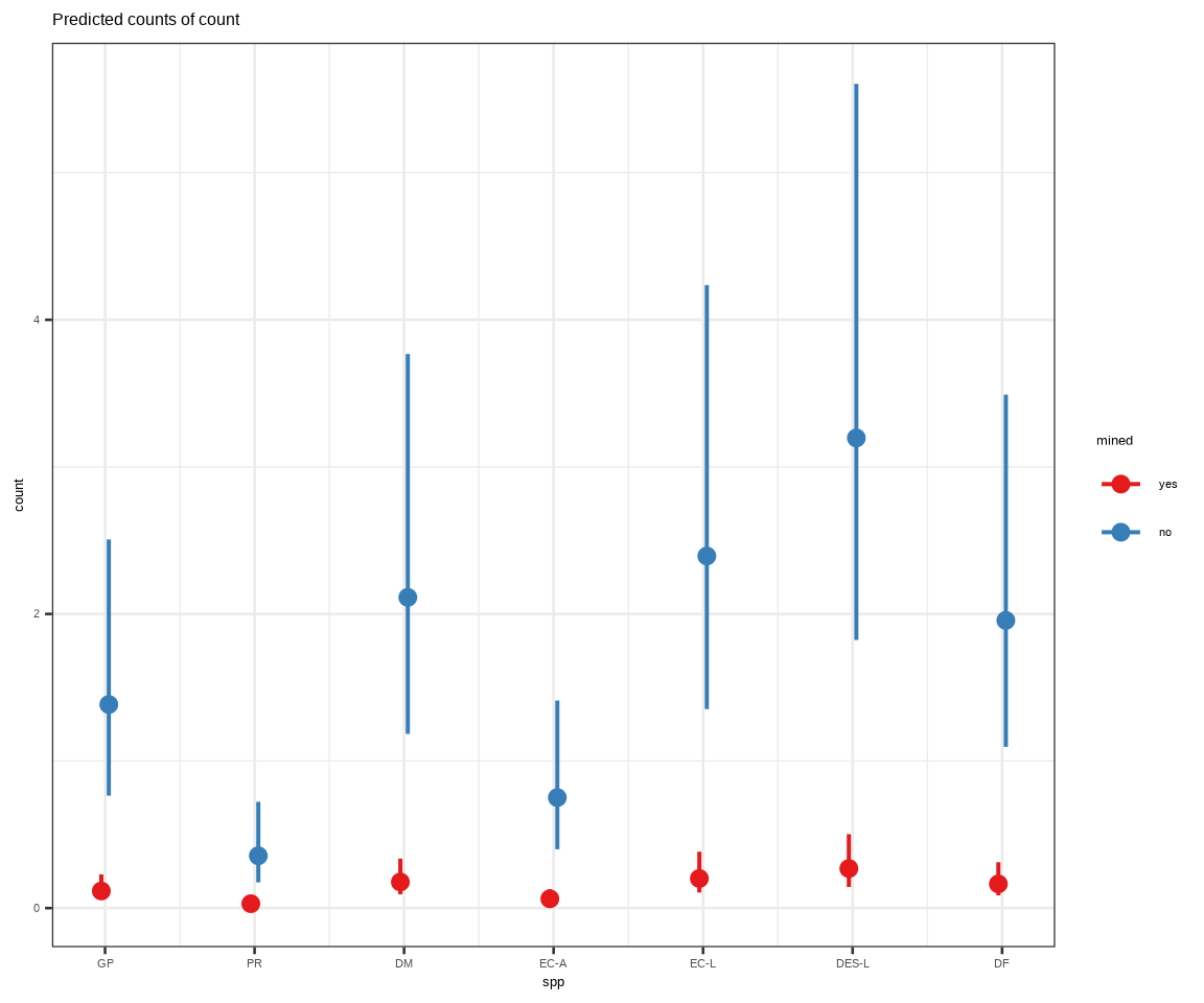
plot_model() of {sjPlot} creates plots from regression models, either estimates (as so-called forest or dot whisker plots) or marginal effects.

Code

plot_model(model_nested, type = "pred", terms = c("spp", "mined"), show.values = TRUE)

You are calculating adjusted predictions on the population-level (i.e.
  `type = "fixed"`) for a *generalized* linear mixed model.
  This may produce biased estimates due to Jensen's inequality. Consider
  setting `bias_correction = TRUE` to correct for this bias.
  See also the documentation of the `bias_correction` argument.

Mixed-Effect Models for Overdispersed Count Data

When analyzing count data, overdispersion is a common issue where the variance of the outcome variable exceeds the mean. This can lead to biased parameter estimates and incorrect inferences if not properly addressed. In this section, we will demonstrate how to fit mixed-effects regression models for overdispersed count data. First we check for overdispersion in the Poisson model and then adjust for overdispersion using the quasi-Poisson approximation or fit a negative binomial model as an alternative.

Check for Overdispersion

Check for overdispersion of model_nested by calculating the ratio of the residual deviance to the degrees of freedom:

Code

# Check overdispersion
overdispersion_ratio <- sum(residuals(model_nested, type = "pearson")^2) / df.residual(model_nested)
cat("Overdispersion ratio:", overdispersion_ratio, "\n")

Overdispersion ratio: 1.153974

If the overdispersion ratio is significantly greater than 1, overdispersion is present.

Or we can use the performance::check_overdispersion() function to check for overdispersion in the model_nested.

Code

performance::check_overdispersion(model_nested)

# Overdispersion test

       dispersion ratio =   1.154
  Pearson's Chi-Squared = 730.465
                p-value =   0.004

Overdispersion detected.

Adjust for Overdispersion in the Poisson Model (Quasi-Poisson Approximation)

The quasi-Poisson approach is used to handle overdispersion (variance greater than the mean) in count data. However, the {lme4} package does not directly support quasi-Poisson models because it is based on maximum likelihood estimation (which does not accommodate quasi-likelihood models). To address overdispersion in a Poisson model, we can adjust the standard errors post hoc using the overdispersion ratio.

Code

# Adjust standard errors for overdispersion
se_adjusted <- sqrt(overdispersion_ratio) * sqrt(diag(vcov(model_nested)))
coef_table <- summary(model_nested)$coefficients
coef_table[, 2] <- se_adjusted  # Replace standard errors
coef_table[, 3] <- coef_table[, 1] / coef_table[, 2]  # Recompute z-values
coef_table[, 4] <- 2 * (1 - pnorm(abs(coef_table[, 3])))  # Recompute p-values

cat("Adjusted Coefficients Table:\n")

Adjusted Coefficients Table:

Code

print(coef_table)

               Estimate Std. Error    z value     Pr(>|z|)
(Intercept) -2.15025576  0.3870789 -5.5550839 2.774785e-08
minedno      2.47548850  0.3940972  6.2814156 3.355041e-10
cover       -0.06995383  0.1926759 -0.3630648 7.165565e-01
sppPR       -1.35817326  0.4234138 -3.2076736 1.338133e-03
sppDM        0.42274244  0.3564944  1.1858319 2.356887e-01
sppEC-A     -0.61106262  0.3846797 -1.5884970 1.121740e-01
sppEC-L      0.54769788  0.3549285  1.5431217 1.228012e-01
sppDES-L     0.83686853  0.3491793  2.3966730 1.654468e-02
sppDF        0.34574647  0.3582840  0.9650067 3.345414e-01

Fit Quasi-Poisson Model

To account for overdispersion, fit a quasi-Poisson model using the glmmPQL() function of {MASS} package. The quasi-Poisson model is a generalized linear mixed model that relaxes the assumption of equal mean and variance in Poisson regression, making it suitable for overdispersed count data.

Code

# Quasi-Poisson mixed-effects model
model_quasi_poisson <- MASS::glmmPQL(count ~ mined + spp + cover,  random = ~1 | site,  
                             data = mf, family = quasipoisson(link='log'))
summary(model_quasi_poisson)

Linear mixed-effects model fit by maximum likelihood
  Data: mf 
  AIC BIC logLik
   NA  NA     NA

Random effects:
 Formula: ~1 | site
        (Intercept) Residual
StdDev:   0.2888095   1.5873

Variance function:
 Structure: fixed weights
 Formula: ~invwt 
Fixed effects:  count ~ mined + spp + cover 
                 Value Std.Error  DF   t-value p-value
(Intercept) -1.4630935 0.2478870 615 -5.902259  0.0000
minedno      2.2211941 0.2489954  20  8.920625  0.0000
sppPR       -1.3862944 0.3439443 615 -4.030578  0.0001
sppDM        0.2305237 0.2060291 615  1.118889  0.2636
sppEC-A     -0.7701082 0.2734303 615 -2.816470  0.0050
sppEC-L      0.6211737 0.1907148 615  3.257082  0.0012
sppDES-L     0.6791609 0.1888278 615  3.596722  0.0003
sppDF        0.0800427 0.2133052 615  0.375250  0.7076
cover       -0.1686904 0.1105425  20 -1.526023  0.1427
 Correlation: 
         (Intr) minedn sppPR  sppDM  spEC-A spEC-L sDES-L sppDF 
minedno  -0.722                                                 
sppPR    -0.278  0.000                                          
sppDM    -0.463  0.000  0.334                                   
sppEC-A  -0.349  0.000  0.252  0.420                            
sppEC-L  -0.500  0.000  0.361  0.602  0.454                     
sppDES-L -0.505  0.000  0.364  0.608  0.458  0.657              
sppDF    -0.447  0.000  0.322  0.538  0.406  0.582  0.587       
cover     0.278 -0.498  0.000  0.000  0.000  0.000  0.000  0.000

Standardized Within-Group Residuals:
        Min          Q1         Med          Q3         Max 
-1.59244712 -0.45929426 -0.32368772  0.09159159  7.69097201 

Number of Observations: 644
Number of Groups: 23

Fit a Negative Binomial Model (Alternative for Overdispersion)

Negative binomial regression models extend the framework of Poisson regression by addressing a critical limitation inherent in the Poisson approach: the assumption that the variance of the outcome variable is equal to its mean. This assumption can often lead to poor model fit, especially when the data exhibit overdispersion — where the observed variance significantly exceeds the mean. By allowing for greater flexibility in modeling the relationship between the dependent and independent variables, negative binomial regression provides a robust alternative when dealing with count data that do not conform to the strict requirements of the Poisson distribution, making it particularly useful in real-world scenarios where data often show considerable variability.

A negative binomial model can handle overdispersion more directly. First we use {glmmTMB} to fit a negative binomial models. Two parameterisations are often used to fit negative binomial regression models (see Hilbe (2011Hilbe, Joseph M. 2011. Negative Binomial Regression. Cambridge University Press. https://doi.org/10.1017/CBO9780511973420.)):

NB1 (variance = $μ$ + $αμ$); and,
NB2 (variance = $μ+αμ^2$); where $μ$ is the mean, and αα is the overdispersion parameter

NB1 Parameterization

Code

# Negative binomial mixed-effects model
model_negbinom_01 <- glmmTMB(count ~ mined + spp + cover+(1 | site / spp), 
                          data = mf, 
                          family = nbinom1)
# model summary
summary(model_negbinom_01)

 Family: nbinom1  ( log )
Formula:          count ~ mined + spp + cover + (1 | site/spp)
Data: mf

      AIC       BIC    logLik -2*log(L)  df.resid 
   1629.9    1683.5    -802.9    1605.9       632 

Random effects:

Conditional model:
 Groups   Name        Variance Std.Dev.
 spp:site (Intercept) 0.3073   0.5544  
 site     (Intercept) 0.1647   0.4059  
Number of obs: 644, groups:  spp:site, 161; site, 23

Dispersion parameter for nbinom1 family (): 1.49 

Conditional model:
            Estimate Std. Error z value Pr(>|z|)    
(Intercept)  -1.6532     0.3070  -5.386 7.22e-08 ***
minedno       2.2005     0.3058   7.197 6.16e-13 ***
sppPR        -1.3761     0.3633  -3.788 0.000152 ***
sppDM         0.3283     0.2734   1.201 0.229783    
sppEC-A      -0.7819     0.3222  -2.427 0.015221 *  
sppEC-L       0.4735     0.2687   1.762 0.078099 .  
sppDES-L      0.7033     0.2649   2.655 0.007923 ** 
sppDF         0.2610     0.2770   0.942 0.346101    
cover        -0.1140     0.1475  -0.773 0.439301    
---
Signif. codes:  0 '***' 0.001 '**' 0.01 '*' 0.05 '.' 0.1 ' ' 1

NB2 Parameterization

Code

# Negative binomial mixed-effects model
model_negbinom_02 <- glmmTMB(count ~ mined + spp + cover+(1 | site / spp), 
                          data = mf, 
                          family = nbinom2)


# model summary
summary(model_negbinom_02)

 Family: nbinom2  ( log )
Formula:          count ~ mined + spp + cover + (1 | site/spp)
Data: mf

      AIC       BIC    logLik -2*log(L)  df.resid 
   1650.0    1703.6    -813.0    1626.0       632 

Random effects:

Conditional model:
 Groups   Name        Variance Std.Dev.
 spp:site (Intercept) 0.5600   0.7483  
 site     (Intercept) 0.2683   0.5180  
Number of obs: 644, groups:  spp:site, 161; site, 23

Dispersion parameter for nbinom2 family (): 1.67 

Conditional model:
            Estimate Std. Error z value Pr(>|z|)    
(Intercept) -2.06868    0.35949  -5.754 8.69e-09 ***
minedno      2.46956    0.36903   6.692 2.20e-11 ***
sppPR       -1.35107    0.38895  -3.474 0.000513 ***
sppDM        0.42454    0.32716   1.298 0.194398    
sppEC-A     -0.61800    0.35345  -1.748 0.080382 .  
sppEC-L      0.55120    0.32545   1.694 0.090326 .  
sppDES-L     0.83912    0.32031   2.620 0.008801 ** 
sppDF        0.35093    0.32904   1.067 0.286191    
cover       -0.07243    0.18063  -0.401 0.688424    
---
Signif. codes:  0 '***' 0.001 '**' 0.01 '*' 0.05 '.' 0.1 ' ' 1

Code

anova(model_negbinom_01, model_negbinom_02)

Data: mf
Models:
model_negbinom_01: count ~ mined + spp + cover + (1 | site/spp), zi=~0, disp=~1
model_negbinom_02: count ~ mined + spp + cover + (1 | site/spp), zi=~0, disp=~1
                  Df    AIC    BIC  logLik deviance Chisq Chi Df Pr(>Chisq)
model_negbinom_01 12 1629.9 1683.5 -802.93   1605.9                        
model_negbinom_02 12 1650.0 1703.6 -812.99   1626.0     0      0          1

Code

performance::performance(model_negbinom_02)

# Indices of model performance

AIC      |     AICc |      BIC | R2 (cond.) | R2 (marg.) |   ICC |  RMSE
------------------------------------------------------------------------
1649.982 | 1650.477 | 1703.595 |      0.790 |      0.552 | 0.530 | 1.833

AIC      | Sigma | Score_log | Score_spherical
----------------------------------------------
1649.982 | 1.674 |    -1.101 |           0.033

Code

MuMIn::r.squaredGLMM(model_negbinom_02)

                R2m       R2c
delta     0.5021432 0.7178595
lognormal 0.5524042 0.7897121
trigamma  0.4184650 0.5982339

Using `lme4` Package

We also fit a negative binomial mode using glmer.nb() of {lme4} package but it may be slower and unstable compared to {glmmTMB} package.

Code

# Negative binomial mixed-effects model
model_negbinom_03 <- glmer.nb(count ~ mined + spp + cover+(1 | site / spp), 
                          data = mf)

Warning in checkConv(attr(opt, "derivs"), opt$par, ctrl = control$checkConv, :
Model failed to converge with max|grad| = 0.0127471 (tol = 0.002, component 1)

Code

jtools::summ(model_negbinom_03)

Observations	644
Dependent variable	count
Type	Mixed effects generalized linear model
Family	Negative Binomial(1.666)
Link	log

AIC	1648.59
BIC	1702.20
Pseudo-R² (fixed effects)	0.48
Pseudo-R² (total)	0.69

Fixed Effects
	Est.	S.E.	z val.	p
(Intercept)	-2.10	0.36	-5.87	0.00
minedno	2.44	0.36	6.72	0.00
sppPR	-1.34	0.39	-3.44	0.00
sppDM	0.42	0.33	1.29	0.20
sppEC-A	-0.61	0.35	-1.73	0.08
sppEC-L	0.55	0.33	1.68	0.09
sppDES-L	0.83	0.32	2.60	0.01
sppDF	0.35	0.33	1.06	0.29
cover	-0.07	0.18	-0.40	0.69

Random Effects
Group	Parameter	Std. Dev.
spp:site	(Intercept)	0.75
site	(Intercept)	0.51

Grouping Variables
Group	# groups	ICC
spp:site	161	0.10
site	23	0.04

Zero-inflated Mixed Effect Models

Zero-inflated models are used to account for excess zeros in count data, which can arise due to a separate process that generates zeros (e.g., structural zeros) in addition to the count process. In zero-inflated models, the data are assumed to come from two different processes: one that generates zeros and one that generates counts. The zero-inflated Poisson model is a mixture model that combines a Poisson distribution for the count data with a point mass at zero for the excess zeros.

Check for `zero-inflation` and `overdispersion` in the model

We can use the performance::check_zeroinflation() function to check for zero-inflation in the nested model (model_nested).

Code

performance::check_zeroinflation(model_nested)

# Check for zero-inflation

   Observed zeros: 387
  Predicted zeros: 341
            Ratio: 0.88

Model is underfitting zeros (probable zero-inflation).

Code

performance::check_overdispersion(model_nested)

# Overdispersion test

       dispersion ratio =   1.154
  Pearson's Chi-Squared = 730.465
                p-value =   0.004

Overdispersion detected.

It lookes like the model is zero-inflated and also overdispersed.

Fit Zero-Inflated Negative Binomial Model

we can also use the glmmTMB::glmmTMB() function to fit a zero-inflated negative binomila mixed-effects model to the Salamanders dataset.

Code

# Zero-inflated negative binomial mixed-effects model
model_zinb <- glmmTMB(count ~ mined + spp + cover + (1 | site / spp), 
                      data = mf, 
                      family = nbinom2, 
                      ziformula = ~1)
# Summary of the model
summary(model_zinb)

 Family: nbinom2  ( log )
Formula:          count ~ mined + spp + cover + (1 | site/spp)
Zero inflation:         ~1
Data: mf

      AIC       BIC    logLik -2*log(L)  df.resid 
   1652.0    1710.1    -813.0    1626.0       631 

Random effects:

Conditional model:
 Groups   Name        Variance Std.Dev.
 spp:site (Intercept) 0.5600   0.7483  
 site     (Intercept) 0.2683   0.5180  
Number of obs: 644, groups:  spp:site, 161; site, 23

Dispersion parameter for nbinom2 family (): 1.67 

Conditional model:
            Estimate Std. Error z value Pr(>|z|)    
(Intercept) -2.06871    0.35950  -5.754 8.69e-09 ***
minedno      2.46955    0.36903   6.692 2.20e-11 ***
sppPR       -1.35104    0.38895  -3.474 0.000514 ***
sppDM        0.42456    0.32716   1.298 0.194376    
sppEC-A     -0.61797    0.35345  -1.748 0.080398 .  
sppEC-L      0.55124    0.32545   1.694 0.090307 .  
sppDES-L     0.83915    0.32031   2.620 0.008799 ** 
sppDF        0.35096    0.32904   1.067 0.286152    
cover       -0.07243    0.18063  -0.401 0.688421    
---
Signif. codes:  0 '***' 0.001 '**' 0.01 '*' 0.05 '.' 0.1 ' ' 1

Zero-inflation model:
            Estimate Std. Error z value Pr(>|z|)
(Intercept)   -18.81    3766.15  -0.005    0.996

Code

performance::performance(model_zinb)

# Indices of model performance

AIC      |     AICc |      BIC | R2 (cond.) | R2 (marg.) |   ICC |  RMSE
------------------------------------------------------------------------
1651.982 | 1652.560 | 1710.062 |      0.830 |      0.581 | 0.595 | 1.833

AIC      | Sigma | Score_log | Score_spherical
----------------------------------------------
1651.982 | 1.674 |    -1.162 |           0.032

Code

MuMIn::r.squaredGLMM(model_zinb)

                R2m       R2c
delta     0.5021432 0.7178590
lognormal 0.5524043 0.7897118
trigamma  0.4184648 0.5982332

Summary and Conclusion

This tutorial has thoroughly introduced mixed-effects Poisson models, emphasizing their application in analyzing count data while accounting for both fixed and random effects. We begin by constructing a Mixed-Effects Poisson Model from scratch without relying on external libraries. Next, we fit various types of Poisson models using the {lme4}, {glmmTMB}, and {MASS} packages. The {lme4} package is utilized to fit random-effects Poisson models of varying complexity, including random intercept models, random intercept and slope models, and nested random-effects models. The {glmmTMB} package provides enhanced capabilities by fitting negative binomial models to address overdispersion, a common issue with Poisson data. Finally, the {MASS} package demonstrates how to fit quasi-Poisson and negative binomial models as alternatives for handling overdispersion, offering more flexible modeling approaches.

This tutorial explored mixed-effect Poisson modeling, from manual implementation to leveraging powerful R packages. For most practical applications, begin with {lme4} for basic mixed-effects Poisson models. For datasets with overdispersion or more complex structures, consider {glmmTMB} or {MASS} for extended modeling capabilities. By mastering these techniques, you can effectively analyze count data with hierarchical structures, making informed inferences and predictions in various fields such as biostatistics, epidemiology, and ecology.

3.4. Mutilevel or Mixed Effect Poisson Model (MLPM)

Overview

Multilevel Poisson Model from Scratch

Simulated Hierarchical Data

Log-Likelihood Function

Optimize Parameters using optim() and fit the model

Extract Results

Multilevel Poisson Model in R

Install Required R Packages

Load Packages

Data

Goodness-of-fit Tests

Mixed Effect Poisson Models

Fixed-Effects Poisson Model

Random-Intercept Model

Random-Intercept and Slope Model

Nested Random-Effects Model

Compare Models

Model Summary

Model Performance

Marginal Effects and Adjusted Predictions

Mixed-Effect Models for Overdispersed Count Data

Check for Overdispersion

Adjust for Overdispersion in the Poisson Model (Quasi-Poisson Approximation)

Fit Quasi-Poisson Model

Fit a Negative Binomial Model (Alternative for Overdispersion)

NB1 Parameterization

NB2 Parameterization

Using lme4 Package

Zero-inflated Mixed Effect Models

Check for zero-inflation and overdispersion in the model

Fit Zero-Inflated Negative Binomial Model

Summary and Conclusion

References

Optimize Parameters using `optim()` and fit the model

Using `lme4` Package

Check for `zero-inflation` and `overdispersion` in the model