Code
cubic_spline_basis <- function(x, knots) {
  X <- cbind(1, x, x^2, x^3)  # Polynomial terms up to cubic
  for (knot in knots) {
    X <- cbind(X, pmax(0, (x - knot)^3))  # Truncated cubic splines at each knot
  }
  return(X)
}![]()

Generalized Additive Models (GAMs) are powerful tools for modeling complex, nonlinear relationships in data. They combine the flexibility of nonparametric models with the interpretability of linear models. This tutorial will guide you through the fundamentals of GAMs in R. To enhance your understanding, we will build a GAM model from scratch without using any external packages. This approach will illustrate the core principles behind GAM modeling, including smoothing, combining predictor effects, and estimating model parameters. We will also explore various packages for fitting, analyzing, and visualizing GAMs, including popular libraries such as {mgcv} and {gam}. These packages provide robust functions to fit GAMs, offering flexibility with multiple types of smoothers, diagnostics, and model selection criteria. Additionally, we will delve into specific packages designed for GAM visualization and model assessment, equipping you with tools to evaluate and interpret complex relationships in your data.
By the end of this tutorial, you will have a comprehensive understanding of how to use GAMs in R to uncover intricate relationships in your data. You will gain practical skills in fitting, interpreting, and diagnosing GAM models, along with insights into the mathematical principles behind them.
A Generalized Additive Model (GAM) is an extension of traditional linear regression models that allows for more flexibility by modeling the relationship between the response variable and each predictor variable as a smooth, non-linear function. This flexibility makes GAMs especially useful when relationships between predictors and the outcome are complex and cannot be adequately captured by a linear model.
1. Structure of a GAM
A Generalized Additive Model (GAM) is defined as:
\[ g(E(y)) = \beta_0 + f_1(x_1) + f_2(x_2) + \dots + f_n(x_n) \]
where:
In GAMs, instead of assuming each predictor affects the outcome linearly, each predictor has its own flexible function, allowing it to influence the outcome in potentially complex, nonlinear ways.
2. Components of a GAM
To better understand GAMs, let’s look at the main components:
Each predictor \(x_i\) has its own smooth function, \(f_i(x_i)\), which is designed to capture the potentially nonlinear relationship between \(x_i\) and \(y\)). These functions are often estimated using methods like:
These smoothing methods help model the relationship between each predictor and the outcome in a flexible, data-driven way.
The link function \(g\) relates the predictors to the expected value of \(y\). Some commonly used link functions are:
Identity Link: \(g(y) = y\), used for continuous outcomes (e.g., linear regression).
Log Link: \(g(y) = \ln(y)\), used for modeling positive, skewed outcomes like counts.
Logit Link: \(g(y) = \ln\left(\frac{y}{1 - y}\right)\), used for binary or proportion data.
By choosing an appropriate link function, GAMs can model different types of outcome distributions (continuous, binary, count data, etc.).
GAMs assume that each predictor contributes independently to the outcome, meaning there are no interactions between predictors (although it’s possible to add interaction terms). This additivity makes GAMs interpretable because we can examine the effect of each predictor individually.
3. Estimation and Fitting GAMs
To estimate a GAM, the following steps are typically involved:
Each smooth function \(f_i(x_i)\) needs to be tuned for “smoothness.” If \(f_i(x_i)\) is too flexible, the model might overfit the data, capturing noise rather than true relationships. Conversely, if \(f_i(x_i)\) is too rigid, it may miss important trends. Regularization methods, such as penalizing the complexity of \(f_i(x_i)\), help control this balance. The degree of smoothness is often chosen by minimizing a model selection criterion like Generalized Cross-Validation (GCV) or Akaike Information Criterion (AIC).
The coefficients \(\beta_0\) and the functions \(f_i(x_i)\) are estimated by maximizing the likelihood of the model (or minimizing a loss function). This is often done using iterative algorithms, like backfitting, that alternate between fitting each function while keeping the others fixed until convergence.
Once fitted, a GAM can be evaluated using: - Residual analysis: Plotting residuals to check for patterns, which can indicate model misfit. - Cross-validation: Splitting data into training and test sets to check predictive performance. - Model selection criteria: Metrics like AIC or GCV to compare different model specifications.
4. Benefits and Limitations of GAMs
5. Applications of GAMs
In ecology, GAMs are often used to study the relationship between species abundance and environmental factors (e.g., temperature, rainfall). For example, one might model how fish population changes with water temperature, salinity, and nutrient levels in a non-linear manner.
In economics, GAMs can model relationships that are not strictly linear, like how consumer spending varies with income level and Income. GAMs allow each of these factors to influence spending in complex, nonlinear ways.
In medical research, GAMs are used to model the effects of Income, dosage levels, or other health metrics on patient outcomes, where the relationship might be nonlinear (e.g., the effect of dosage on blood pressure might increase up to a point and then level off).
In marketing, GAMs are useful to understand how advertising spend, customer demographics, and other factors impact customer engagement or sales, which often have nonlinear effects.
To develop a Generalized Additive Model (GAM) with 4 predictors from scratch in R, we’ll apply cubic spline basis functions to each predictor independently. This will allow each predictor to have a non-linear effect on the outcome variable. We’ll also include a regularization term to prevent overfitting. The model will be fit using least squares optimization.
Certainly! I’ll walk you through creating a Generalized Additive Model (GAM) from scratch without using any GAM-specific functions. This will include generating the spline basis, calculating coefficients, computing predictions, residuals, model summary statistics, and evaluating performance through cross-validation. Let’s break down the steps in detail.
For each predictor, we’ll create a cubic spline basis matrix with num_knots. We’ll use this basis for the GAM.
cubic_spline_basis <- function(x, knots) {
X <- cbind(1, x, x^2, x^3) # Polynomial terms up to cubic
for (knot in knots) {
X <- cbind(X, pmax(0, (x - knot)^3)) # Truncated cubic splines at each knot
}
return(X)
}Next, we construct the full design matrix by generating spline basis functions for each predictor and concatenating them.
create_design_matrix <- function(data, predictors, num_knots) {
  X_spline <- NULL
  spline_list <- list()  # To store each predictor's spline basis

  for (predictor in predictors) {
    x <- data[[predictor]]
    knots <- seq(min(x), max(x), length.out = num_knots)  # Equally spaced knots
    X_spline_predictor <- cubic_spline_basis(x, knots)  # Generate spline basis
    spline_list[[predictor]] <- X_spline_predictor
    X_spline <- cbind(X_spline, X_spline_predictor)  # Append to design matrix
  }

  return(list(X_spline = X_spline, spline_list = spline_list))
}Here, we add a small regularization term \(\lambda\) to ensure the matrix \(X^T X\) is invertible, then solve for the coefficients.
fit_gam_model <- function(X_spline, y, lambda = 0.0001) {
  XtX <- t(X_spline) %*% X_spline + lambda * diag(ncol(X_spline))  # Regularization
  Xty <- t(X_spline) %*% y
  coefficients <- solve(XtX, Xty)  # Solve for coefficients
  return(coefficients)
}With the coefficients, we can predict the outcome for the training data.
predict_gam <- function(X_spline, coefficients) {
  y_pred <- X_spline %*% coefficients
  return(y_pred)
}After fitting, we’ll calculate residuals, deviance, and mean squared error to summarize model fit.
compute_summary_stats <- function(y, y_pred) {
  residuals <- y - y_pred
  deviance <- sum(residuals^2)  # Residual Sum of Squares
  mse <- mean(residuals^2)      # Mean Squared Error

  return(list(residuals = residuals, deviance = deviance, mse = mse))
}We’ll estimate each predictor’s effect by fitting sub-models with each individual predictor’s spline matrix.
compute_anova_table <- function(data, response, predictors, spline_list, lambda = 0.0001) {
  anova_table <- data.frame(
    Predictor = predictors,
    Sum_of_Squares = sapply(predictors, function(predictor) {
      X_pred <- spline_list[[predictor]]
      XtX_single <- t(X_pred) %*% X_pred + lambda * diag(ncol(X_pred))
      Xty_single <- t(X_pred) %*% data[[response]]
      coefficients_single <- solve(XtX_single, Xty_single)
      residuals_single <- data[[response]] - X_pred %*% coefficients_single
      return(sum(residuals_single^2))
    })
  )
  return(anova_table)
}We’ll use k-fold cross-validation to estimate model performance on unseen data. Here’s the cross-validation setup:
cross_validate_gam <- function(data, response, predictors, num_knots = 3, lambda = 0.0001, k_folds = 5) {
  n <- nrow(data)
  fold_size <- n %/% k_folds
  indices <- sample(n)
  mse_folds <- numeric(k_folds)

  for (fold in 1:k_folds) {
    # Define training and validation sets
    validation_idx <- indices[((fold - 1) * fold_size + 1):(fold * fold_size)]
    train_data <- data[-validation_idx, ]
    validation_data <- data[validation_idx, ]

    # Create design matrix for training data
    train_design <- create_design_matrix(train_data, predictors, num_knots)
    X_train <- train_design$X_spline
    y_train <- train_data[[response]]

    # Fit the model on training data
    coefficients <- fit_gam_model(X_train, y_train, lambda)

    # Design matrix for validation data
    validation_design <- create_design_matrix(validation_data, predictors, num_knots)
    X_val <- validation_design$X_spline
    y_val <- validation_data[[response]]

    # Predict on validation set and calculate MSE
    y_val_pred <- predict_gam(X_val, coefficients)
    mse_folds[fold] <- mean((y_val - y_val_pred)^2)
  }

  cv_mse <- mean(mse_folds)  # Average MSE over folds
  return(cv_mse)
}Let’s fit the GAM model on synthetic data and show summary results, ANOVA table, and cross-validation performance.
# Set up data and parameters
set.seed(0)
n_samples <- 100
data <- data.frame(
  x1 = seq(0, 10, length.out = n_samples),
  x2 = runif(n_samples, 0, 10),
  x3 = runif(n_samples, 0, 10),
  x4 = runif(n_samples, 0, 10)
)
data$y <- 3 * sin(data$x1) + 2 * log(data$x2 + 1) - 1.5 * sqrt(data$x3) + 0.5 * data$x4^2 +
  rnorm(n_samples, mean = 0, sd = 0.5)

predictors <- c("x1", "x2", "x3", "x4")
response <- "y"
num_knots <- 4
lambda <- 0.0001

# Create design matrix
design_matrix <- create_design_matrix(data, predictors, num_knots)
X_spline <- design_matrix$X_spline
spline_list <- design_matrix$spline_list

# Fit model and make predictions
coefficients <- fit_gam_model(X_spline, data[[response]], lambda)
y_pred <- predict_gam(X_spline, coefficients)

# Calculate summary statistics
summary_stats <- compute_summary_stats(data[[response]], y_pred)

# ANOVA table
anova_table <- compute_anova_table(data, response, predictors, spline_list, lambda)

# Cross-Validation
cv_mse <- cross_validate_gam(data, response, predictors, num_knots, lambda)

# Print results
cat("GAM Summary:\n")
GAM Summary:cat("-----------------------------------------------------\n")-----------------------------------------------------cat("Coefficients:\n")Coefficients:print(coefficients) [,1]
-0.023161388
x 8.271536899
-4.329322919
0.275690380
0.275691755
-0.660576687
-0.203910265
0.000000000
-0.023161443
x 0.613274576
0.203197548
0.001829571
-0.046738682
0.086780236
-0.116798305
0.000000000
-0.023161449
x -1.996700452
0.481026490
0.116913912
-0.174194894
0.061741229
-0.009306572
0.000000000
-0.023161442
x -0.634788449
0.435050301
0.250545657
-0.258615383
-0.003922149
-0.010824794
0.000000000cat("\nMean Squared Error:", round(summary_stats$mse, 4), "\n")
Mean Squared Error: 0.4349 cat("Deviance:", round(summary_stats$deviance, 4), "\n")Deviance: 43.4897 cat("Residuals:\n")Residuals:print(head(summary_stats$residuals)) [,1]
[1,] 1.19802648
[2,] 0.01107583
[3,] 0.02853082
[4,] 1.18566512
[5,] 0.29919007
[6,] -0.59918471cat("\nANOVA for Parametric Effects:\n")
ANOVA for Parametric Effects:print(anova_table) Predictor Sum_of_Squares
x1 x1 19152.0461
x2 x2 19581.0390
x3 x3 20748.8882
x4 x4 594.4656cat("\nCross-Validated MSE:", round(cv_mse, 4), "\n")
Cross-Validated MSE: 478.6997 This approach builds the GAM model manually from scratch without relying on GAM-specific R packages, and it evaluates performance using cross-validation to check for overfitting or underfitting.
In R, you can fit Generalized Additive Models (GAMs) using different packages, each offering unique functionalities. Here’s a quick guide to fitting GAMs using three popular packages:
mgcv Packagemgcv is the most widely used package for GAMs in R due to its flexibility, efficiency, and support for a wide range of models. It uses penalized regression splines by default.
Key Features: mgcv provides a variety of smooth functions (e.g., s(), te() for tensor product smoothing) and allows you to specify different distributions and link functions using family=.
The gam package (distinct from mgcv) is based on Hastie and Tibshirani’s original GAM framework. It has a simpler interface but is less flexible than mgcv for complex models.
Key Features: The gam package is good for standard GAMs and allows lo() for locally-weighted regression smoothers. It’s simpler but lacks some of the advanced features found in mgcv.
gamlss Packagegamlss (Generalized Additive Models for Location, Scale, and Shape) extends GAMs to model not only the mean (location) but also other parameters (e.g., scale, shape) of the distribution.
Key Features: gamlss is highly flexible for distributional modeling. It supports a wide range of distributions, including non-standard ones, and allows for different smoothers (e.g., pb() for P-splines).
Following R packages are required to run this notebook. If any of these packages are not installed, you can install them using the code below:
packages <- c('tidyverse',
     'plyr',
      'DataExplorer',
         'dlookr',
         'rstatix',
       'flextable',
         'gtsummary',
         'performance',
       'report',
         'sjPlot',
         'margins',
         'marginaleffects',
         'ggeffects',
       'ggpmisc',
         'patchwork',
         'metrica',
         'MASS',
       'gam',
         'gamair',
         'mgcv',
         'gamlss',
         'gratia',
         #'itsadug',  # we will load this pacakge later
         'agridat'
        )
#| warning: false
#| error: false
# Install missing packages
new_packages <- packages[!(packages %in% installed.packages()[,"Package"])]
if(length(new_packages)) install.packages(new_packages)
# Verify installation
cat("Installed packages:\n")
print(sapply(packages, requireNamespace, quietly = TRUE))# Load packages with suppressed messages
invisible(lapply(packages, function(pkg) {
suppressPackageStartupMessages(library(pkg, character.only = TRUE))
}))# Check loaded packages
cat("Successfully loaded packages:\n")Successfully loaded packages:print(search()[grepl("package:", search())]) [1] "package:agridat" "package:gratia"
[3] "package:gamlss" "package:parallel"
[5] "package:gamlss.dist" "package:gamlss.data"
[7] "package:mgcv" "package:nlme"
[9] "package:gamair" "package:gam"
[11] "package:foreach" "package:splines"
[13] "package:MASS" "package:metrica"
[15] "package:patchwork" "package:ggpmisc"
[17] "package:ggpp" "package:ggeffects"
[19] "package:marginaleffects" "package:margins"
[21] "package:sjPlot" "package:report"
[23] "package:performance" "package:gtsummary"
[25] "package:flextable" "package:rstatix"
[27] "package:dlookr" "package:DataExplorer"
[29] "package:plyr" "package:lubridate"
[31] "package:forcats" "package:stringr"
[33] "package:dplyr" "package:purrr"
[35] "package:readr" "package:tidyr"
[37] "package:tibble" "package:ggplot2"
[39] "package:tidyverse" "package:stats"
[41] "package:graphics" "package:grDevices"
[43] "package:utils" "package:datasets"
[45] "package:methods" "package:base" In this exercise, we utilize a dataset that includes average science scores by country from the Programme for International Student Assessment (PISA) conducted in 2006. Alongside these scores, we also consider data from the United Nations, which includes Gross National Income (GNI) per capita (adjusted for Purchasing Power Parity in 2005 dollars), the Educational Index, the Health Index, and the Human Development Index (HDI).
The education component is measured by the mean years of schooling for adults aged 25 years and older and the expected years of schooling for children of school entry Income. The health index is determined by life expectancy at birth, while the wealth component is based on GNI per capita. The HDI establishes minimum and maximum values for each dimension, with the resulting scores indicating each country’s position relative to these endpoints, expressed as a value between 0 and 1.
The key variables are as follows (variable abbreviations in bold):
Overall Science Score (average score for 15 year olds)
Interest in science
Identifying scientific Issues
Explaining phenomena scientifically
Support for scientific inquiry
Income Index
Health Index
Education Index
Human Development Index (composed of the Income index, Health Index, and Education Index)
We will use read_csv() function of {readr} package to import data as a tidy data.
# Load data
mf<-readr::read_csv("https://raw.githubusercontent.com/m-clark/generalized-additive-models/master/data/pisasci2006.csv")
# Remove missing values
mf<-na.omit(mf)
str(mf)
tibble [52 × 11] (S3: tbl_df/tbl/data.frame)
$ Country : chr [1:52] "Argentina" "Australia" "Austria" "Belgium" ...
$ Overall : num [1:52] 391 527 511 510 390 434 534 438 542 388 ...
$ Issues : num [1:52] 395 535 505 515 398 427 532 444 528 402 ...
$ Explain : num [1:52] 386 520 516 503 390 444 531 432 549 379 ...
$ Evidence: num [1:52] 385 531 505 516 378 417 542 440 542 383 ...
$ Interest: num [1:52] 567 465 507 503 592 523 469 591 536 644 ...
$ Support : num [1:52] 506 487 515 492 519 527 501 564 529 546 ...
$ Income : num [1:52] 0.678 0.826 0.835 0.831 0.637 0.663 0.84 0.673 0.853 0.616 ...
$ Health : num [1:52] 0.868 0.965 0.944 0.935 0.818 0.829 0.951 0.923 0.966 0.829 ...
$ Edu : num [1:52] 0.786 0.978 0.824 0.868 0.646 0.778 0.902 0.764 0.763 0.624 ...
$ HDI : num [1:52] 0.773 0.92 0.866 0.877 0.695 0.753 0.897 0.78 0.857 0.683 ...
- attr(*, "na.action")= 'omit' Named int [1:13] 1 5 29 30 33 36 42 43 50 51 ...
..- attr(*, "names")= chr [1:13] "1" "5" "29" "30" ...The key variables are as follows (variable abbreviations in bold):
Overall Science Score (average score for 15 year olds)
Interest in science
Identifying scientific Issues
Explaining phenomena scientifically
Support for scientific inquiry
Income Index
Health Index
Education Index
Human Development Index (composed of the Income index, Health Index, and Education Index)
We can use {ggplot2} to create a scatterplot matrix to visualize the relationships between the variables in the dataset.
# create a data frame with the variables of interest
df<-mf |>
  dplyr::select(Country, Overall,Income, Health,  Edu, Interest)
# create a scatter plot  qith smooth line
p1<-ggplot(df, aes(x = Overall, y = Income)) +
  geom_point() +
  geom_smooth(method = "gam", formula = y ~ splines::bs(x, 4), se = TRUE)
p2<-ggplot(df, aes(x = Overall, y = Health)) +
  geom_point() +
  geom_smooth(method = "gam", formula = y ~ splines::bs(x, 4), se = TRUE)
p3<-ggplot(df, aes(x = Overall, y = Edu)) +
  geom_point() +
  geom_smooth(method = "gam", formula = y ~ splines::bs(x, 4), se = TRUE)
p4<-ggplot(df, aes(x = Overall, y = Interest)) +
  geom_point() +
  geom_smooth(method = "gam", formula = y ~ splines::bs(x, 4), se = TRUE)
library(patchwork)
(p1+p2)/(p3+p4)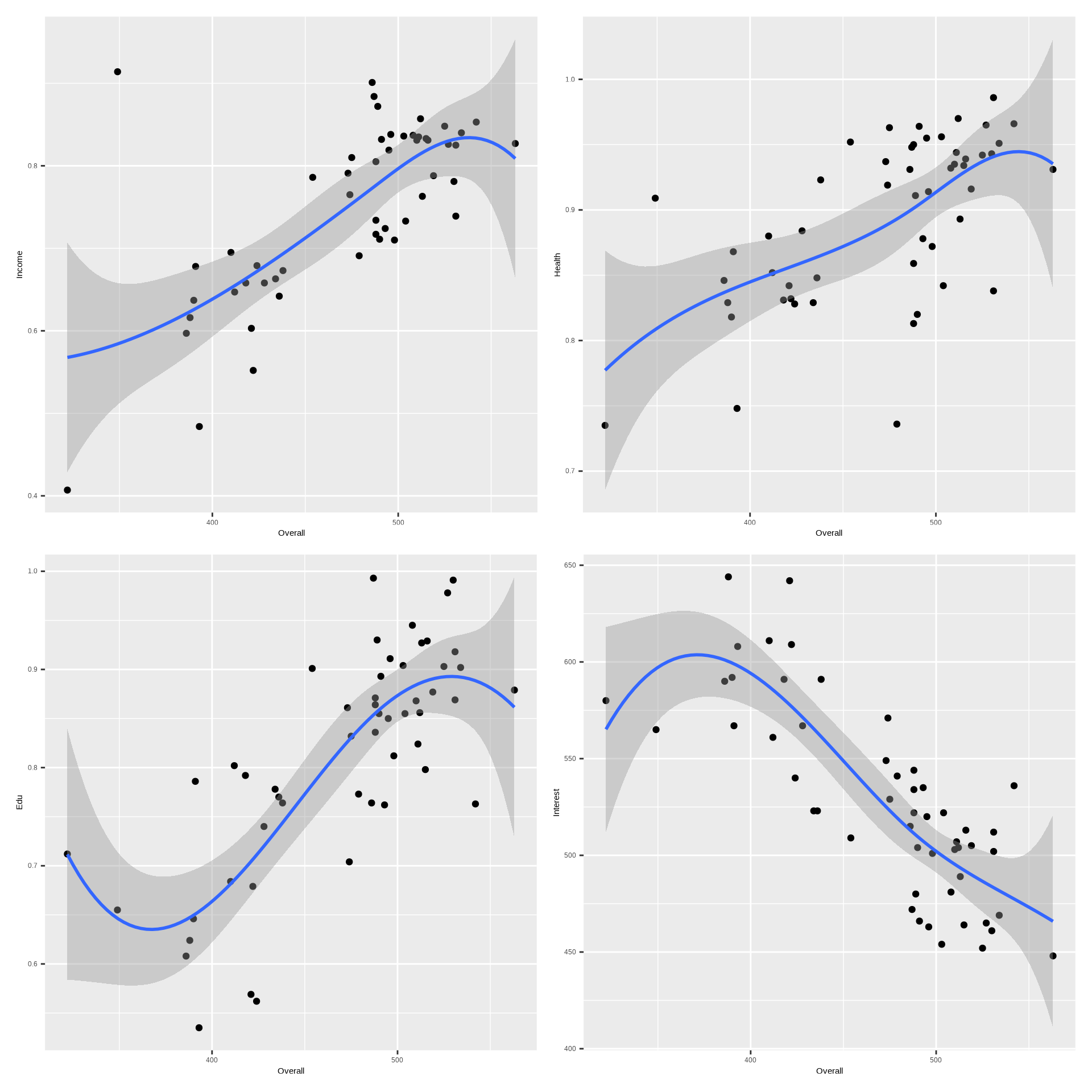
The scatterplot matrix shows relationships between the four important variables in the Overall dataset. For example, the scatterplot of Overall vs. all for prectors reveals a non-linear relationship, suggesting a GAM might be appropriate.
We will split the data into training and testing sets, The training set will contain 70% of the data, and the testing set will contain the remaining 30%.
# set the seed to make your partition reproducible
seeds = 11076
## 75% of the sample size
smp_size <- floor(0.75 * nrow(mf))
## set the seed to make your partition reproducible
set.seed(123)
train_ind <- sample(seq_len(nrow(mf)), size = smp_size)
train <- mf[train_ind, ]
test <- mf[-train_ind, ]In this example, we’ll fit a univariate GAM model using the {mgcv}, {gam}, and {gamlss} packages to model the relationship between the Overall variable and a single predictor Income of Overall data set. We’ll use a cubic regression spline with 3 degrees of freedom. We will use s() is the shorthand for fitting smoothing splines in gam() function.
{gam} function is used to fit a GAM model in the {mgcv} package. The s() function is used to specify a smooth term for the predictor Income using a cubic regression spline. family() object specifying the distribution and link to use in fitting etc.
library(mgcv)
# Fit a GAM model using the mgcv package
mgcv.uni <- mgcv::gam(Overall ~ s(Income), data = train,
              family= gaussian(link = "identity"))
summary(mgcv.uni)
Family: gaussian
Link function: identity

Formula:
Overall ~ s(Income)

Parametric coefficients:
            Estimate Std. Error t value Pr(>|t|)
(Intercept)  472.718      3.953   119.6   <2e-16 ***
---
Signif. codes:  0 '***' 0.001 '**' 0.01 '*' 0.05 '.' 0.1 ' ' 1

Approximate significance of smooth terms:
            edf Ref.df     F p-value
s(Income) 7.585   8.49 20.47  <2e-16 ***
---
Signif. codes:  0 '***' 0.001 '**' 0.01 '*' 0.05 '.' 0.1 ' ' 1

R-sq.(adj) =  0.817   Deviance explained = 85.3%
GCV = 781.25  Scale est. = 609.28    n = 39
summary(mgcv.uni) provides a summary of the fitted GAM model, including the estimated coefficients, degrees of freedom, and significance levels for each term. The edf column shows the effective degrees of freedom for the smooth term, which is a measure of the complexity of the fitted curve. The p-value column indicates the significance of the smooth term in the model. In this case, the smooth term for Income is highly significant (p < 0.001), suggesting that Income has a non-linear effect on Overall. The R-sq.(adj) value represents the adjusted R-squared value of the model, which is a measure of how well the model fits the data. In this case, the adjusted R-squared value is 0.817, indicating that the model explains 81% of the variance in Overall.
The {gratia} package is designed to work with {mgcv} and offers enhanced visualization and diagnostic tools.
# Enhanced visualization
gratia::draw(mgcv.uni) # Generates nicely formatted plots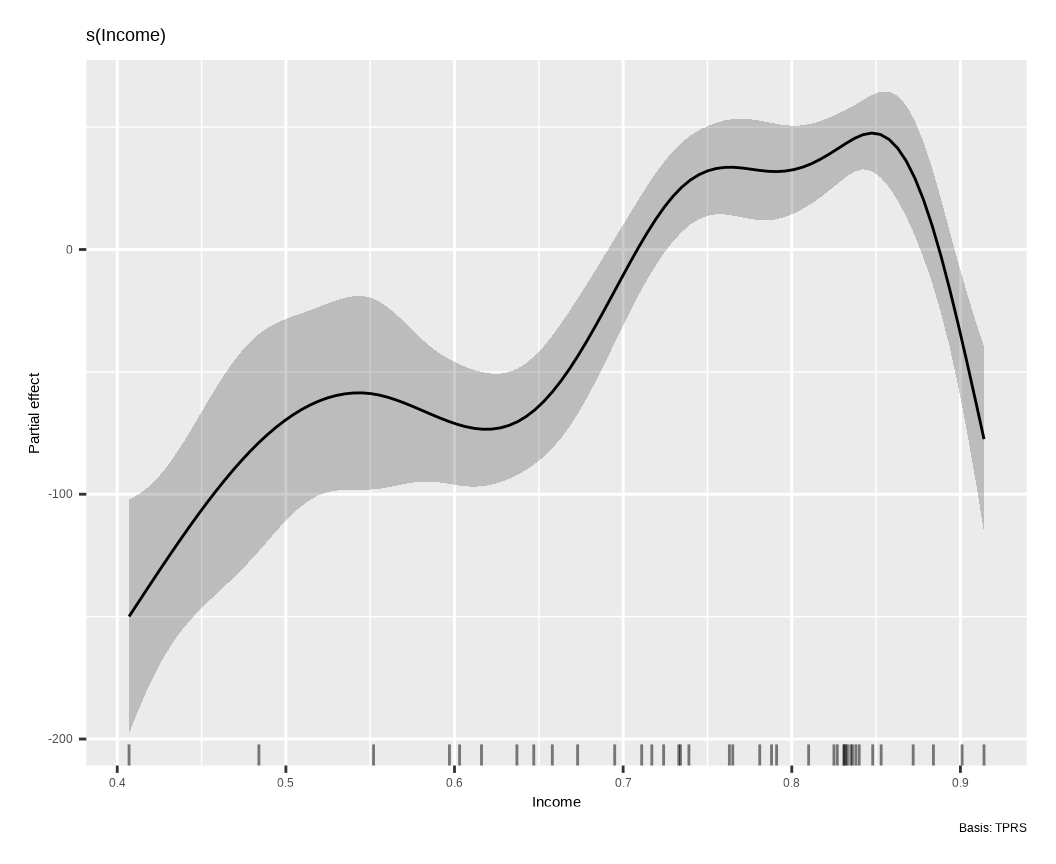
The {gam} package provides a simpler interface for fitting GAMs. The gam() function is used to fit a GAM model with a cubic regression spline for the predictor Income. The s() function is used to specify a smooth term for the predictor Income using a cubic regression spline.
##  you have to detach {mgcv} before using {gam} package
detach("package:mgcv", unload=F)
# Fit a GAM to model the relationship between mpg and hp
gam.uni <- gam::gam(Overall ~ s(Income), data = train,
                      family= gaussian(link = "identity"))
# Summary of the GAM
summary(gam.uni)
Call: gam::gam(formula = Overall ~ s(Income), family = gaussian(link = "identity"),
    data = train)
Deviance Residuals:
    Min      1Q  Median      3Q     Max
-94.230 -12.954   3.988  17.807  50.374

(Dispersion Parameter for gaussian family taken to be 845.4251)

    Null Deviance: 126385.9 on 38 degrees of freedom
Residual Deviance: 28744.31 on 33.9998 degrees of freedom
AIC: 380.1803

Number of Local Scoring Iterations: NA

Anova for Parametric Effects
          Df Sum Sq Mean Sq F value   Pr(>F)
s(Income)  1  60339   60339  71.371 7.26e-10 ***
Residuals 34  28744     845
---
Signif. codes:  0 '***' 0.001 '**' 0.01 '*' 0.05 '.' 0.1 ' ' 1

Anova for Nonparametric Effects
            Npar Df Npar F    Pr(F)
(Intercept)
s(Income)         3 14.707 2.63e-06 ***
---
Signif. codes:  0 '***' 0.001 '**' 0.01 '*' 0.05 '.' 0.1 ' ' 1
Above output provides a summary of the fitted GAM model, including the estimated coefficients, degrees of freedom, and significance levels for each term. Anova for parametric effect shows the sum of squares contributed by each predictor. The p-value column indicates the significance of the smooth term in the model. In this case, the smooth term for Income is highly significant (p < 0.001), suggesting that Income has a non-linear effect on Overall.
#Plotting the Model
plot(gam.uni,se = TRUE) 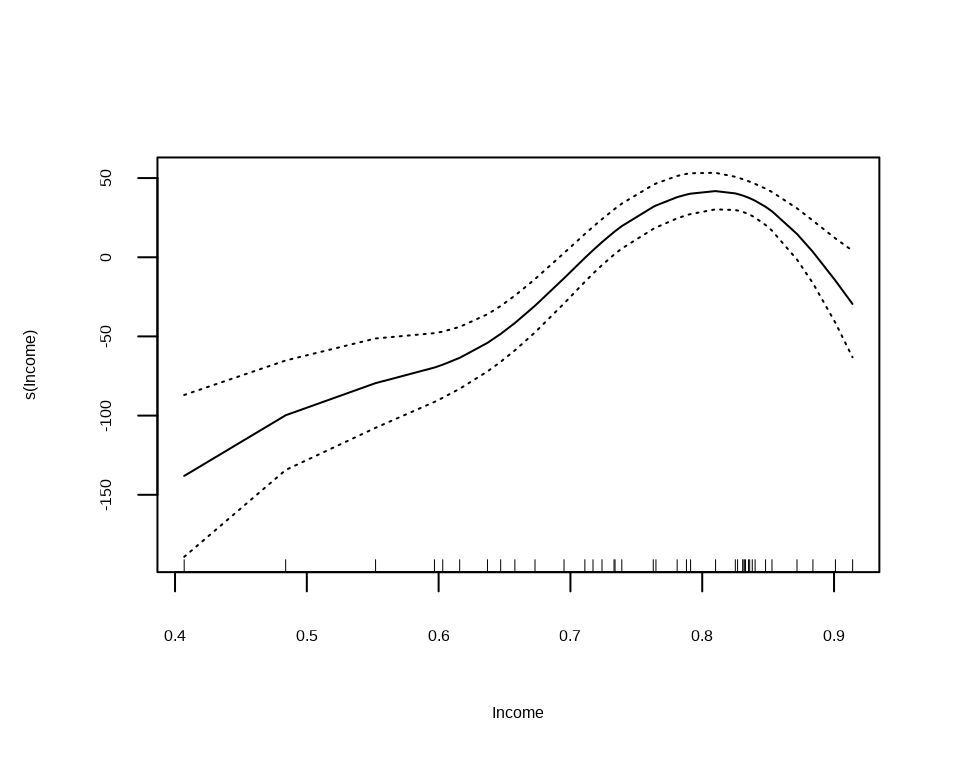
#se stands for standard error Bandgamlss() function fits a Generalized Additive Model for Location, Scale, and Shape (GAMLSS) using the {gamlss} package. This function allows for modeling the entire distribution of the response variable, not just the mean. The distribution for the response variable in the GAMLSS can be selected from a very general family of distributions including highly skew and/or kurtotic continuous and discrete distributions, and the parameters of the distribution can be modeled as functions of covariates.
We will use pb() is the shorthand for fitting smoothing function.
gamlss.uni <- gamlss(Overall ~ pb(Income), data = train, # pb() is a smooth function
                       family =NO) # NO() defines the normal distribution
GAMLSS-RS iteration 1: Global Deviance = 356.9995
GAMLSS-RS iteration 2: Global Deviance = 356.9665
GAMLSS-RS iteration 3: Global Deviance = 356.9672 summary(gamlss.uni)******************************************************************
Family: c("NO", "Normal")
Call: gamlss(formula = Overall ~ pb(Income), family = NO, data = train)
Fitting method: RS()
------------------------------------------------------------------
Mu link function: identity
Mu Coefficients:
Estimate Std. Error t value Pr(>|t|)
(Intercept) 216.19 24.84 8.703 7.77e-10 ***
pb(Income) 342.32 32.77 10.447 1.09e-11 ***
---
Signif. codes: 0 '***' 0.001 '**' 0.01 '*' 0.05 '.' 0.1 ' ' 1
------------------------------------------------------------------
Sigma link function: log
Sigma Coefficients:
Estimate Std. Error t value Pr(>|t|)
(Intercept) 3.1576 0.1132 27.89 <2e-16 ***
---
Signif. codes: 0 '***' 0.001 '**' 0.01 '*' 0.05 '.' 0.1 ' ' 1
------------------------------------------------------------------
NOTE: Additive smoothing terms exist in the formulas:
i) Std. Error for smoothers are for the linear effect only.
ii) Std. Error for the linear terms maybe are not accurate.
------------------------------------------------------------------
No. of observations in the fit: 39
Degrees of Freedom for the fit: 7.927218
Residual Deg. of Freedom: 31.07278
at cycle: 3
Global Deviance: 356.9672
AIC: 372.8216
SBC: 386.009
******************************************************************#Plotting the Model
plot(gamlss.uni,se = TRUE) 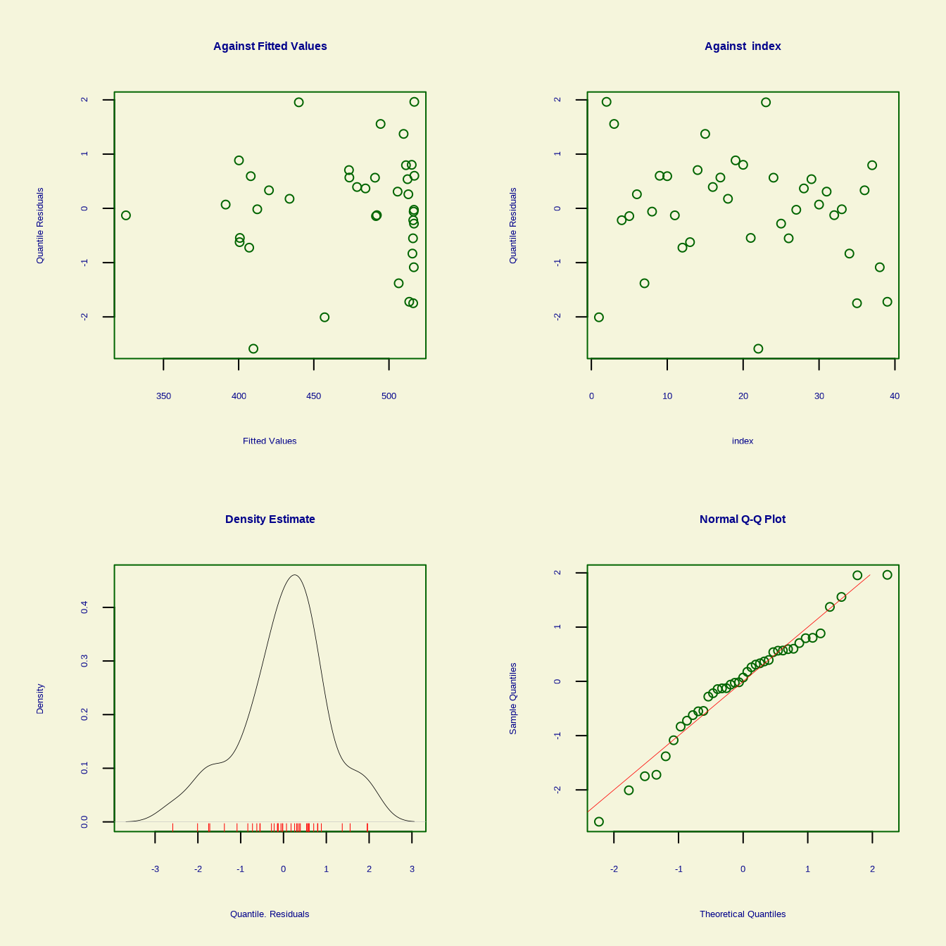
******************************************************************
          Summary of the Quantile Residuals
                           mean   =  -2.890954e-14
                       variance   =  1.026316
               coef. of skewness  =  -0.4128001
               coef. of kurtosis  =  3.077463
Filliben correlation coefficient  =  0.9841758
******************************************************************#se stands for standard error BandTo fit a multivariate Generalized Additive Model (GAM) using the Overall dataset from the {ISLR} package in R, we can approach this using the {mgcv}, {gam}, and {gamlss} packages. We will model the relationship between the Overall variable and multiple predictors: Income, Edu, Health and Interest. We will use cubic regression splines for each predictor.
{gam} function is used to fit a GAM model in the {mgcv} package. The s() function is used to specify a smooth term for the predictors Income, Edu, Health and interest using a cubic regression spline. k is the number of knots to use in the basis expansion. The default is 10. The k argument controls the smoothness of the fitted curve. We use k=15 for each predictor.
library(mgcv)
# Fit a GAM model using the mgcv package
mgcv.multi <- mgcv::gam(Overall ~ s(Income, k=15) + s(Edu, k=15) + s(Health, k=15) + s(Interest, k=15), data = train,
              family= gaussian(link = "identity"))
summary(mgcv.multi)
Family: gaussian
Link function: identity

Formula:
Overall ~ s(Income, k = 15) + s(Edu, k = 15) + s(Health, k = 15) +
    s(Interest, k = 15)

Parametric coefficients:
            Estimate Std. Error t value Pr(>|t|)
(Intercept)  472.718      2.582   183.1   <2e-16 ***
---
Signif. codes:  0 '***' 0.001 '**' 0.01 '*' 0.05 '.' 0.1 ' ' 1

Approximate significance of smooth terms:
              edf Ref.df     F p-value
s(Income)   5.894  6.915 4.799 0.00356 **
s(Edu)      7.022  8.216 1.914 0.11761
s(Health)   2.099  2.519 0.618 0.54811
s(Interest) 5.131  6.081 2.276 0.08152 .
---
Signif. codes:  0 '***' 0.001 '**' 0.01 '*' 0.05 '.' 0.1 ' ' 1

R-sq.(adj) =  0.922   Deviance explained = 96.3%
GCV = 567.73  Scale est. = 259.92    n = 39
Above output provides a summary of the fitted GAM model, including the estimated coefficients, degrees of freedom, and significance levels for each term. The effective degrees of freedom (edf) column shows the effective degrees of freedom for the smooth term, which is a measure of the complexity of the fitted curve. The p-value column indicates the significance of the smooth term in the model. In this case, the smooth term for Income and Interest are highly significant (p < 0.001), suggesting that both these predictors have a non-linear effect on Overall. The R-sq.(adj) value represents the adjusted R-squared value of the model, which is a measure of how well the model fits the data. In this case, the adjusted R-squared value is 0.92, indicating that the model explains 92% of the variance in Overall. The GCV, or generalized cross validation score can be taken as an estimate of the mean square prediction error based on a leave-one-out cross validation estimation process.
The {gratia} package is designed to work with {mgcv} and offers enhanced visualization and diagnostic tools.
# Enhanced visualization
gratia::draw(mgcv.multi) # Generates nicely formatted plots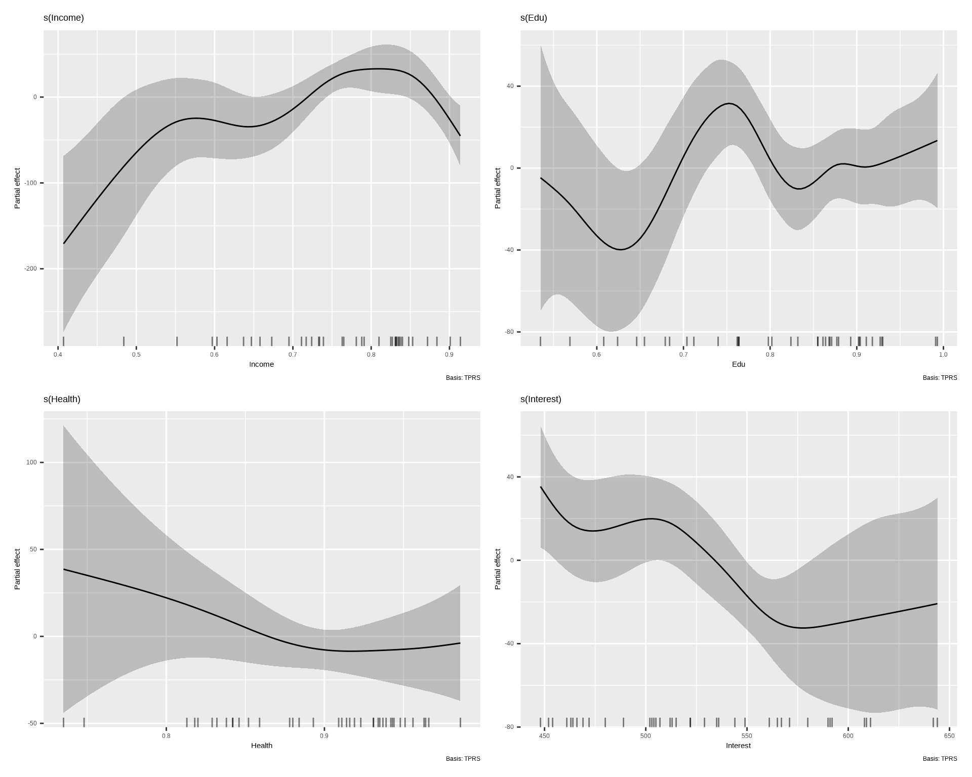
Plot revels the fitted GAM model, including the smooth terms for Income, Edu, Health, and Interest. The solid lines represent the estimated relationships between each predictor and Overall, while the shaded areas represent the 95% confidence intervals around the estimates. The plot shows non-linear relationships between each predictor and Overall, with different patterns for each predictor. The smooth terms capture these non-linear relationships effectively.
The {gam} package provides a simpler interface for fitting GAMs. The gam() function is used to fit a GAM model with a cubic regression spline for the predictor Income, Edu, Health and Interest. df is the degree of freedom for the spline.
##  you have to detach {mgcv} before using {gam} package
detach("package:mgcv", unload=TRUE)
# Fit a GAM to model the relationship between mpg and hp
gam.multi <- gam::gam(Overall ~ s(Income, df=15) + s(Edu, df=15) + s(Health, df=15) + s(Interest, df=15),  data = train,
                      family= gaussian(link = "identity"))
# Summary of the GAM
summary(gam.multi)
Call: gam::gam(formula = Overall ~ s(Income, df = 15) + s(Edu, df = 15) +
    s(Health, df = 15) + s(Interest, df = 15), family = gaussian(link = "identity"),
    data = train)

(Dispersion Parameter for gaussian family taken to be Inf)

    Null Deviance: 126385.9 on 38 degrees of freedom
Residual Deviance: 349.6113 on -21.9994 degrees of freedom
AIC: 320.2131

Number of Local Scoring Iterations: NA

Anova for Parametric Effects
                          Df Sum Sq Mean Sq   F value Pr(>F)
s(Income, df = 15)     1.000  53505   53505 -3366.803    NaN
s(Edu, df = 15)        1.000   2017    2017  -126.917    NaN
s(Health, df = 15)     1.000   1562    1562   -98.317    NaN
s(Interest, df = 15)   1.000   4731    4731  -297.707    NaN
Residuals            -21.999    350     -16

Anova for Nonparametric Effects
                     Npar Df Npar F Pr(F)
(Intercept)
s(Income, df = 15)        14      0
s(Edu, df = 15)           14      0
s(Health, df = 15)        14      0
s(Interest, df = 15) 14 0 #Plotting the Model
par(mfrow=c(2,2)) #to partition the Plotting Window
plot(gam.multi) 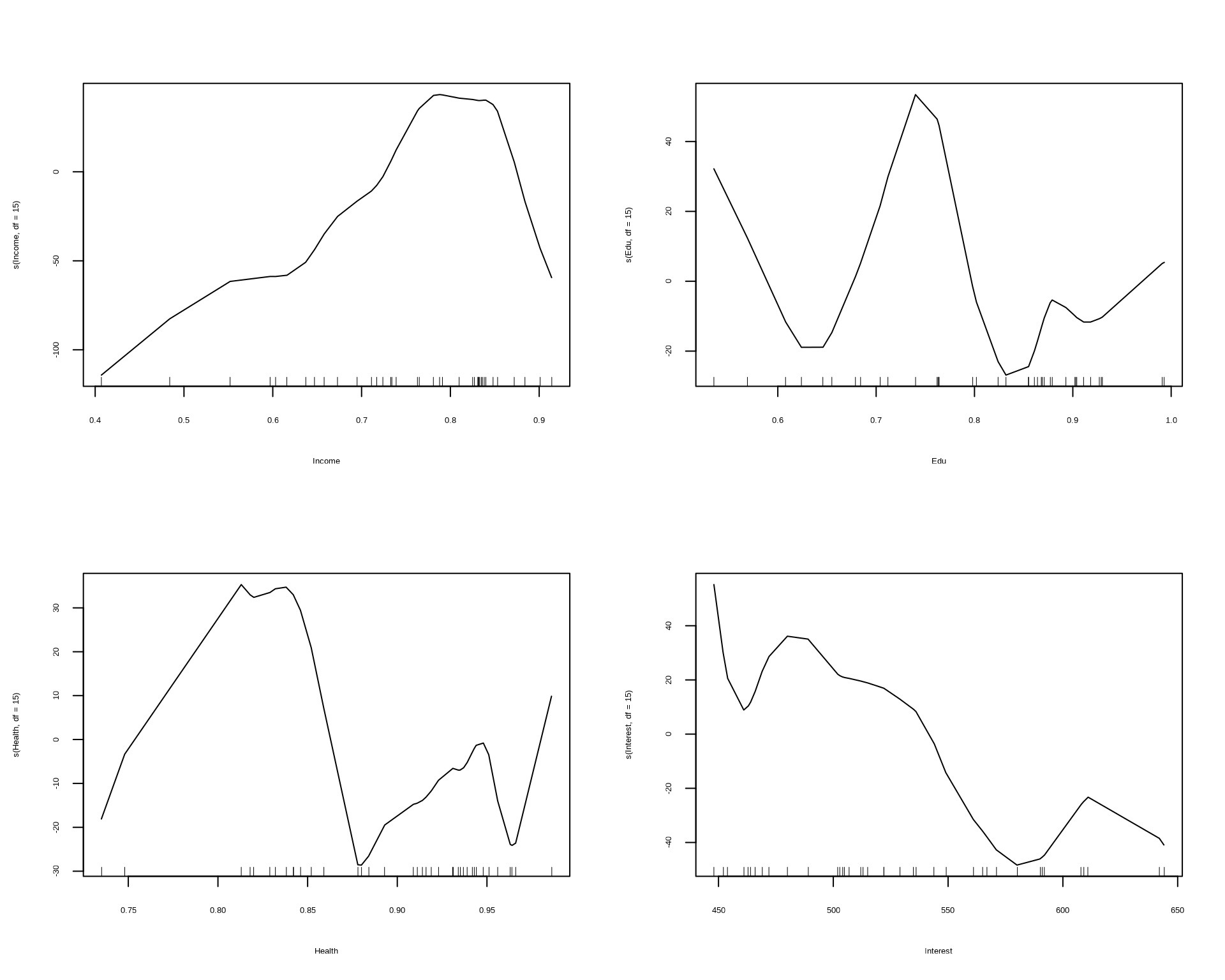
#se stands for standard error Bandgamlss() function fits a Generalized Additive Model for Location, Scale, and Shape (GAMLSS) using the {gamlss} package. This function allows for modeling the entire distribution of the response variable, not just the mean. The distribution for the response variable in the GAMLSS can be selected from a very general family of distributions including highly skew and/or kurtotic continuous and discrete distributions, and the parameters of the distribution can be modeled as functions of covariates.
We will use pb() is the shorthand for fitting smoothing function.
gamlss.multi <- gamlss(Overall ~  pb(Income) + pb(Edu) + pb(Health) + pb(Interest), data = train, # pb() is a smooth function
                       family =NO) # NO() defines the normal distribution
GAMLSS-RS iteration 1: Global Deviance = 350.7869
GAMLSS-RS iteration 2: Global Deviance = 350.7779
GAMLSS-RS iteration 3: Global Deviance = 350.777 summary(gamlss.multi)******************************************************************
Family: c("NO", "Normal")
Call: gamlss(formula = Overall ~ pb(Income) + pb(Edu) + pb(Health) +
pb(Interest), family = NO, data = train)
Fitting method: RS()
------------------------------------------------------------------
Mu link function: identity
Mu Coefficients:
Estimate Std. Error t value Pr(>|t|)
(Intercept) 446.4572 140.8345 3.170 0.00359 **
pb(Income) 165.0185 68.3467 2.414 0.02233 *
pb(Edu) 102.7553 61.0514 1.683 0.10314
pb(Health) 17.9481 112.8828 0.159 0.87478
pb(Interest) -0.3709 0.1446 -2.565 0.01580 *
---
Signif. codes: 0 '***' 0.001 '**' 0.01 '*' 0.05 '.' 0.1 ' ' 1
------------------------------------------------------------------
Sigma link function: log
Sigma Coefficients:
Estimate Std. Error t value Pr(>|t|)
(Intercept) 3.0782 0.1132 27.19 <2e-16 ***
---
Signif. codes: 0 '***' 0.001 '**' 0.01 '*' 0.05 '.' 0.1 ' ' 1
------------------------------------------------------------------
NOTE: Additive smoothing terms exist in the formulas:
i) Std. Error for smoothers are for the linear effect only.
ii) Std. Error for the linear terms maybe are not accurate.
------------------------------------------------------------------
No. of observations in the fit: 39
Degrees of Freedom for the fit: 10.13701
Residual Deg. of Freedom: 28.86299
at cycle: 3
Global Deviance: 350.777
AIC: 371.051
SBC: 387.9146
******************************************************************From above output Global Deviance is 350.7, AIC is 371, BIC is 387.91 and Sigma Coefficients of estimates 3.70 (p<0.001). The p-value column indicates the significance of the smooth term in the model. In this case, the smooth term for Income and Interest are significant (p < 0.05), suggesting that both these predictors have a non-linear effect on Overall.
#Plotting the Model
plot(gamlss.multi,se = TRUE) 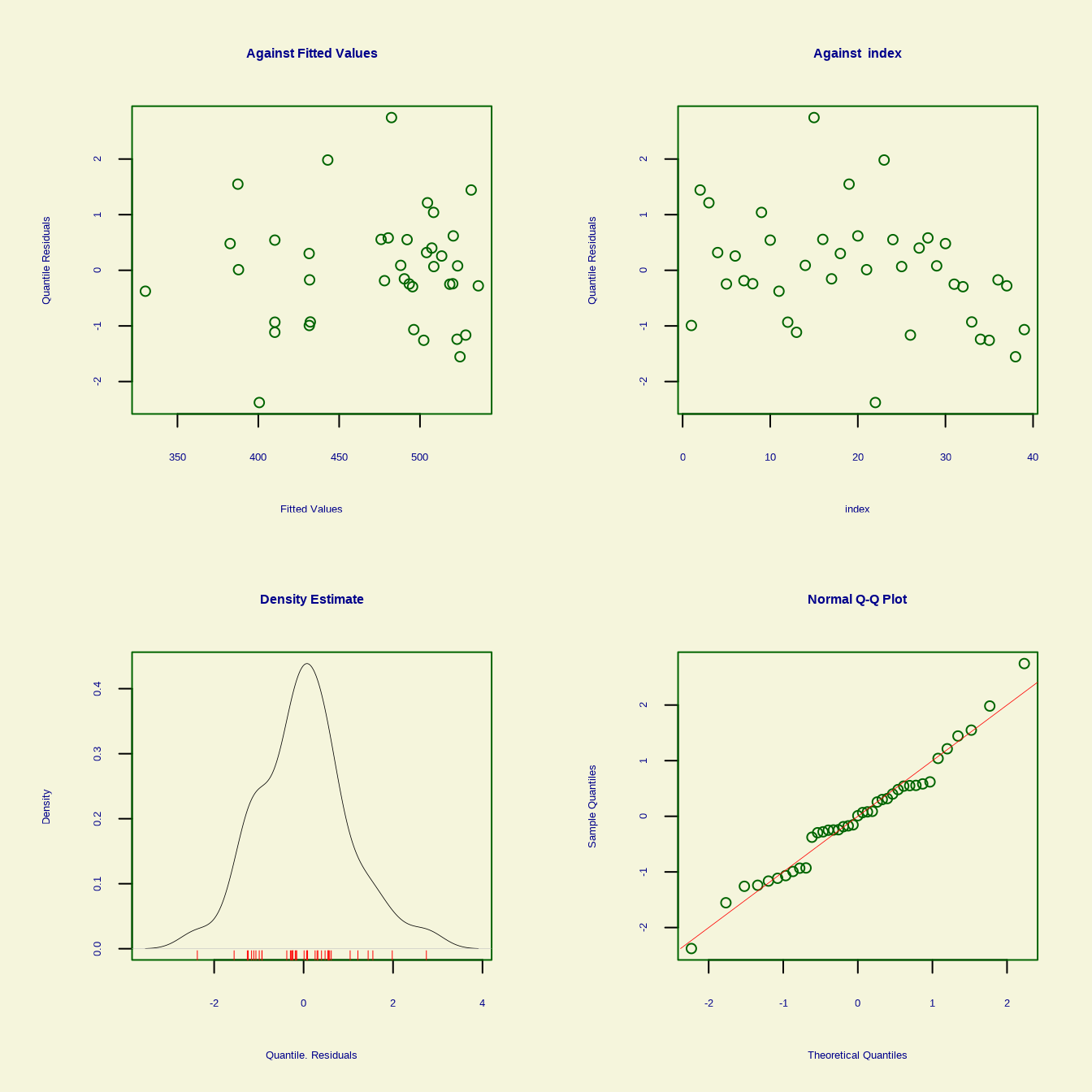
******************************************************************
          Summary of the Quantile Residuals
                           mean   =  -2.013754e-12
                       variance   =  1.026316
               coef. of skewness  =  0.2784542
               coef. of kurtosis  =  3.311798
Filliben correlation coefficient  =  0.986157
******************************************************************#se stands for standard error BandIn the context of the gam() function from the mgcv package in R, smoothing functions (or smooth terms) are tools used to model non-linear relationships between predictors and the response variable. They allow the data to determine the shape of the relationship, rather than assuming a fixed functional form like linear or polynomial.
Common Smoothing Functions in gam():
s():
gam().Example:
gam_model <- gam(y ~ s(x), data = dataset)Options within s():
bs: Specifies the type of basis (default: “tp” for thin plate regression splines).k: Controls the number of basis functions (higher values allow more flexibility).fx: If TRUE, fits a fixed degree of smoothness.by: Allows interaction with a categorical variable.te(): Tensor product smooths
Example:
gam_model <- gam(y ~ te(x1, x2), data = dataset)ti(): Tensor interaction smooth
te() but fits an interaction without the main effects.Example:
gam_model <- gam(y ~ ti(x1, x2), data = dataset)bs="cr" (Cubic Regression Splines):
s().Example:
gam_model <- gam(y ~ s(x, bs = "cr"), data = dataset)bs="cc" (Cyclic Cubic Splines):
Example:
gam_model <- gam(y ~ s(x, bs = "cc"), data = dataset)bs="cs" (Shrinkage Cubic Splines):
Example:
gam_model <- gam(y ~ s(x, bs = "cs"), data = dataset)bs="tp" (Thin plate regression spline (default):
Example: R gam_model <- gam(y ~ s(x, bs = "tp"), data = dataset)
s() with multiple predictors:
s() term.Example:
gam_model <- gam(y ~ s(x1, x2), data = dataset)Key Features of Smoothing in gam():
Automatic Smoothness Selection:
gam() automatically determines the level of smoothness using techniques like generalized cross-validation (GCV) or restricted maximum likelihood (REML).Penalty for Overfitting:
Basis Dimension (k):
s(x, k = 10) uses 10 basis functions.Visualization:
plot().Example:
plot(gam_model, pages = 1)library(mgcv)This is mgcv 1.9-1. For overview type 'help("mgcv-package")'.
Attaching package: 'mgcv'The following objects are masked from 'package:gam':
gam, gam.control, gam.fit, s# Thin plate regression spline
gam.tp <- gam(Overall ~ s(Income, bs="tp", k=15) +
s(Edu, bs="tp", k=15) +
s(Health, bs="tp", k=15) +
s(Interest, bs="tp", k=15),
method="REML",
data = train)
# Cubic regression spline
gam.cr <- gam(Overall ~ s(Income, bs="cr", k=15) +
s(Edu, bs="cr", k=15) +
s(Health, bs="cr", k=15) +
s(Interest, bs="cr", k=15),
method="REML",
data = train)
# cubic-spline.
gam.cc <- gam(Overall ~ s(Income, bs="cc", k=15) +
s(Edu, bs="cc", k=15) +
s(Health, bs="cc", k=15) +
s(Interest, bs="cc", k=15),
method="REML",
data = train)# Compare models using AIC
AIC(gam.tp, gam.cr, gam.cc) df AIC
gam.tp 14.56445 368.0780
gam.cr 14.24128 368.0626
gam.cc 13.68113 378.5195The effective degrees of freedom (EDF) gives a sense of the smoothness of each term. Higher EDF values indicate a more flexible curve, while lower values indicate more smoothing.
summary(gam.tp)$edf[1] 4.606812 1.000123 1.000094 3.926832summary(gam.cr)$edf[1] 4.496544 1.000095 1.000075 3.866270summary(gam.cc)$edf[1] 4.3625195598 2.2771086909 0.0001987258 2.3567049719Use the {itsadug} package to compare different models with varied smooth terms automatically.
This package has the compareML() function to automatically compare a set of candidate models and select the one with the lowest AIC or other model selection criteria.
library(itsadug)Loading required package: plotfunctions
Attaching package: 'plotfunctions'The following object is masked from 'package:ggplot2':
alphaLoaded package itsadug 2.4 (see 'help("itsadug")' ).
Attaching package: 'itsadug'The following object is masked from 'package:gratia':
dispersionThe following object is masked from 'package:ggeffects':
get_predictions# Compare models
compareML(gam.cr, gam.tp)gam.cr: Overall ~ s(Income, bs = "cr", k = 15) + s(Edu, bs = "cr", k = 15) +
s(Health, bs = "cr", k = 15) + s(Interest, bs = "cr", k = 15)
gam.tp: Overall ~ s(Income, bs = "tp", k = 15) + s(Edu, bs = "tp", k = 15) +
s(Health, bs = "tp", k = 15) + s(Interest, bs = "tp", k = 15)
Model gam.cr preferred: lower REML score (5.597), and equal df (0.000).
-----
Model Score Edf Difference Df
1 gam.tp 168.7726 9
2 gam.cr 163.1753 9 5.597 0.000
AIC difference: -0.02, model gam.cr has lower AIC.compareML(gam.cr, gam.cc)gam.cr: Overall ~ s(Income, bs = "cr", k = 15) + s(Edu, bs = "cr", k = 15) +
s(Health, bs = "cr", k = 15) + s(Interest, bs = "cr", k = 15)
gam.cc: Overall ~ s(Income, bs = "cc", k = 15) + s(Edu, bs = "cc", k = 15) +
s(Health, bs = "cc", k = 15) + s(Interest, bs = "cc", k = 15)
Chi-square test of REML scores
-----
Model Score Edf Difference Df p.value Sig.
1 gam.cc 189.1265 5
2 gam.cr 163.1753 9 25.951 4.000 1.446e-10 ***
AIC difference: -10.46, model gam.cr has lower AIC.Use purrr::map to loop over different smoothing functions and assess the best fit based on AIC or GCV. This method allows you to test several different smoothing options and select the best model.
In gam(), set the method to "REML" or "GCV.Cp" to let the model choose smoothing parameters that minimize either REML (restricted maximum likelihood) or GCV (generalized cross-validation) criteria.
REML is typically preferred because it often leads to smoother fits than GCV and is more stable in terms of penalizing overfitting.
# List of smoothing basis types to test
smooth_types <- c("tp", "cr", "cc")

# Fit models with each type of smooth and calculate AIC
models <- purrr::map(smooth_types, ~ gam(Overall ~
            s(Income, bs = .x) +
            s(Edu, bs = .x) +
            s(Health, bs =.x) +
            s(Interest, bs =.x),
            data = train,
            method = "REML"))


aic_values <- map_dbl(models, AIC)

# Find the best model by minimum AIC
best_model <- models[[which.min(aic_values)]]
summary(best_model)
Family: gaussian
Link function: identity

Formula:
Overall ~ s(Income, bs = .x) + s(Edu, bs = .x) + s(Health, bs = .x) +
    s(Interest, bs = .x)

Parametric coefficients:
            Estimate Std. Error t value Pr(>|t|)
(Intercept)  472.718      2.965   159.4   <2e-16 ***
---
Signif. codes:  0 '***' 0.001 '**' 0.01 '*' 0.05 '.' 0.1 ' ' 1

Approximate significance of smooth terms:
              edf Ref.df     F p-value
s(Income)   5.237  6.117 5.454 0.00133 **
s(Edu)      5.068  5.919 1.834 0.13561
s(Health)   1.603  1.948 0.182 0.80486
s(Interest) 3.249  3.996 1.680 0.19019
---
Signif. codes:  0 '***' 0.001 '**' 0.01 '*' 0.05 '.' 0.1 ' ' 1

R-sq.(adj) =  0.897   Deviance explained = 93.8%
-REML = 164.75  Scale est. = 342.87    n = 39
The {gratia} package is designed to work with {mgcv} and offers enhanced visualization and diagnostic tools.
# Enhanced visualization
gratia::draw(best_model) # Generates nicely formatted plots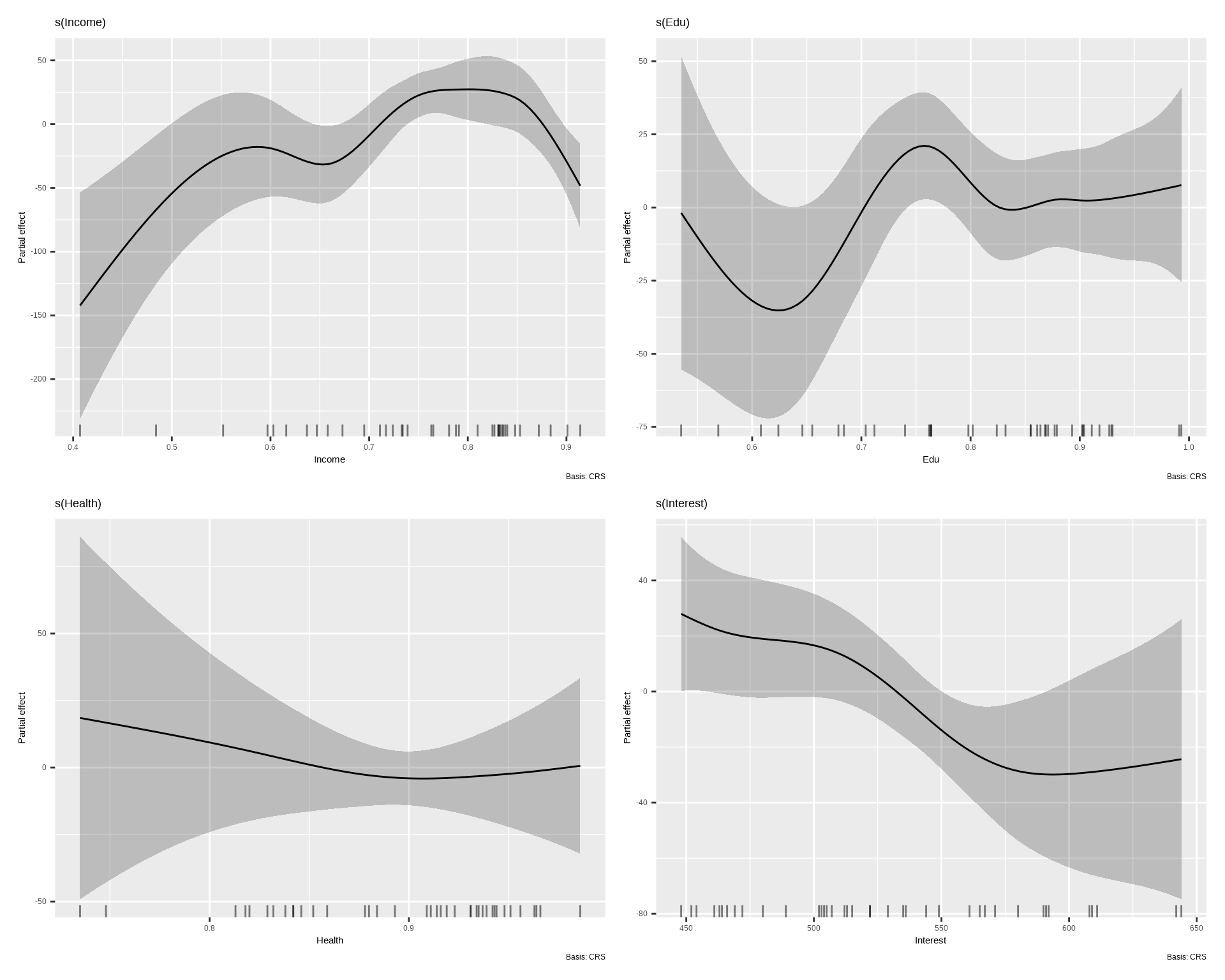
performance::performance(best_model)# Indices of model performance
AIC | AICc | BIC | R2 | RMSE | Sigma
-----------------------------------------------------
357.432 | 403.950 | 390.668 | 0.897 | 14.172 | 18.517The predict() function will be used to predict the Overall Score at the test data. This will help to validate the accuracy of the GAM model.
# Predict the Overall Score at the test data
test$Pred.Overall<-as.data.frame(predict(best_model, newdata = test, type = "response", se=TRUE))

# Compute the MSE
mse <- mean((test$Overall- test$Pred.Overall$fit)^2)
print(paste("MSE:", round(mse, 4)))
[1] "MSE: 679.0869"We can plot observed and predicted values with fitted regression line with {ggplot2} and {ggpmisc} packages.
# load the ggpmisc package
library(ggpmisc)
formula<-y~x
# Plot the observed vs predicted Overall Scores
ggplot(test, aes(Overall,Pred.Overall$fit)) +
  geom_point() +
  geom_smooth(method = "lm")+
  stat_poly_eq(use_label(c("eq", "adj.R2")), formula = formula) +
  ggtitle("GAM: Obs vs Predicted Overal Scores ") +
  xlab("Observed") + ylab("Predicted") +
  scale_x_continuous(limits=c(350,550), breaks=seq(350, 550, 50))+
  scale_y_continuous(limits=c(350,550), breaks=seq(350, 550, 50)) +
  # Flip the bars
  theme(
    panel.background = element_rect(fill = "grey95",colour = "gray75",size = 0.5, linetype = "solid"),
    axis.line = element_line(colour = "grey"),
    plot.title = element_text(size = 14, hjust = 0.5),
    axis.title.x = element_text(size = 14),
    axis.title.y = element_text(size = 14),
    axis.text.x=element_text(size=13, colour="black"),
    axis.text.y=element_text(size=13,angle = 90,vjust = 0.5, hjust=0.5, colour='black'))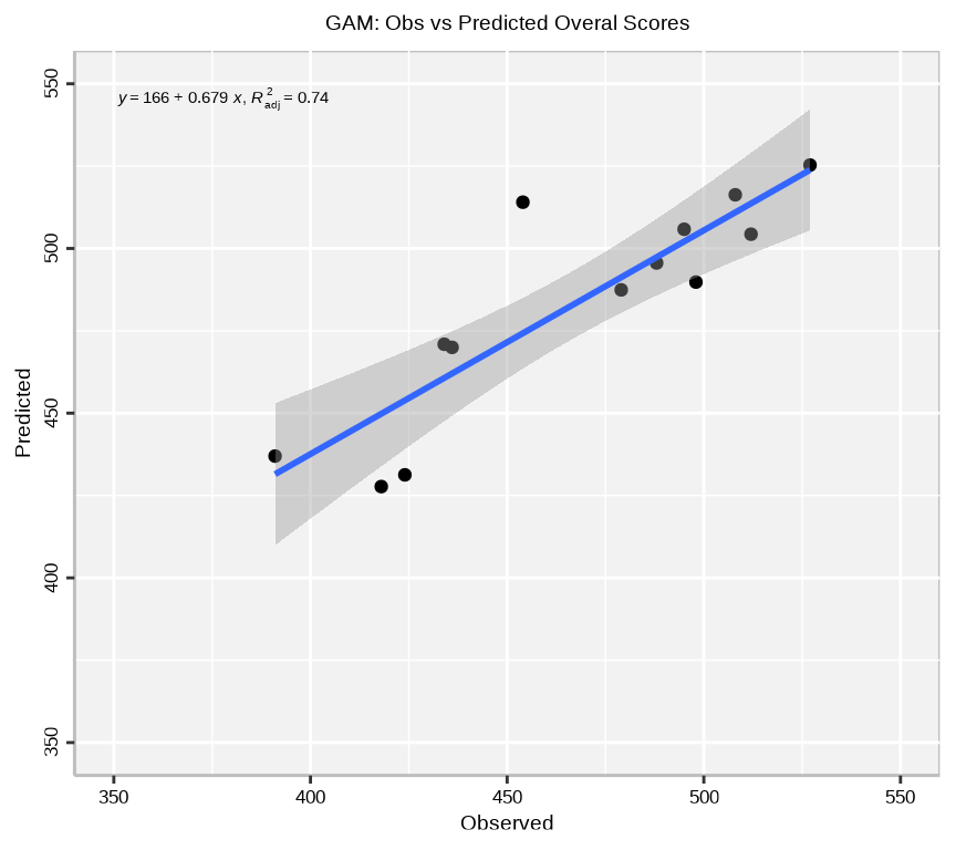
The plot shows the observed Overall Scores on the x-axis and the predicted Overall Scores on the y-axis. The points represent the observed values, while the line represents the fitted regression line. The equation of the regression line and the adjusted R-squared value are displayed on the plot. The plot shows a strong positive relationship between the observed and predicted Overall Scores, indicating that the GAM model is able to accurately predict the Overall Scores.
test<-test |>
  dplyr::mutate(lower = Pred.Overall$fit - 1.96 * Pred.Overall$se.fit,
         upper = Pred.Overall$fit + 1.96 * Pred.Overall$se.fit)

ggplot(aes(x = Income, y = Pred.Overall$fit), data = test) +
  geom_ribbon(aes(ymin = lower, ymax = upper), fill = 'gray92') +
  geom_line(color = '#56B4E9')+
xlab("Income") + ylab("Predicted Overall Scores") 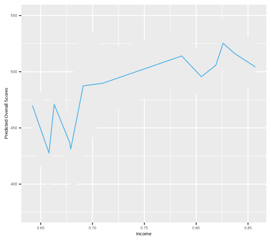
The plot shows the predicted Overall Scores as a function of Income, with a 95% confidence interval around the estimate. The shaded area represents the 95% confidence interval, while the line represents the estimated relationship between Income and Overall Scores. The plot shows a non-linear relationship between Income and Overall Scores, with the Overall Scores increasing with Income up to a certain point and then leveling off.
In this example, we will fit a Poisson regression model to the johnson.blight dataset of {agridat} packages. A data frame with 25 observations on Potato blight due to weather in Prosser, Washington.
binary.data<-agridat::johnson.blight
glimpse(binary.data)
Rows: 25
Columns: 6
$ year <int> 1970, 1971, 1972, 1973, 1974, 1975, 1976, 1977, 1978, 1979, 1…
$ area <int> 0, 0, 0, 0, 50, 810, 120, 40, 0, 0, 0, 0, 10100, 14150, 150, …
$ blight <int> 0, 0, 0, 0, 1, 1, 1, 1, 0, 0, 0, 0, 1, 1, 1, 0, 0, 0, 0, 0, 1…
$ rain.am <int> 8, 9, 9, 6, 16, 10, 12, 10, 11, 8, 13, 8, 15, 9, 17, 5, 8, 5,…
$ rain.ja <int> 1, 4, 6, 1, 6, 7, 12, 4, 10, 9, 1, 3, 6, 12, 1, 4, 3, 5, 3, 8…
$ precip.m <dbl> 5.84, 6.86, 47.29, 8.89, 7.37, 5.08, 3.30, 11.44, 14.99, 4.06…# Define indicator for blight in previous year
binary.data$blight.prev[2:25] <-binary.data$blight[1:24]
binary.data$blight.prev[1] <- 0 # Need this to match the results of Johnson
binary.data$blight.prev <- factor(binary.data$blight.prev)
binary.data$blight <- factor(binary.data$blight)
glimpse(binary.data)Rows: 25
Columns: 7
$ year <int> 1970, 1971, 1972, 1973, 1974, 1975, 1976, 1977, 1978, 1979…
$ area <int> 0, 0, 0, 0, 50, 810, 120, 40, 0, 0, 0, 0, 10100, 14150, 15…
$ blight <fct> 0, 0, 0, 0, 1, 1, 1, 1, 0, 0, 0, 0, 1, 1, 1, 0, 0, 0, 0, 0…
$ rain.am <int> 8, 9, 9, 6, 16, 10, 12, 10, 11, 8, 13, 8, 15, 9, 17, 5, 8,…
$ rain.ja <int> 1, 4, 6, 1, 6, 7, 12, 4, 10, 9, 1, 3, 6, 12, 1, 4, 3, 5, 3…
$ precip.m <dbl> 5.84, 6.86, 47.29, 8.89, 7.37, 5.08, 3.30, 11.44, 14.99, 4…
$ blight.prev <fct> 0, 0, 0, 0, 0, 1, 1, 1, 1, 0, 0, 0, 0, 1, 1, 1, 0, 0, 0, 0… logit.glm = glm(blight ~ blight.prev+rain.am + rain.ja + precip.m, data=binary.data, family=binomial)
logit.gam = gam(blight ~ blight.prev+s(rain.am, rain.ja,k=5) + s(precip.m), data=binary.data, family=binomial) anova(logit.glm, logit.gam, test="Chi") Analysis of Deviance Table
Model 1: blight ~ blight.prev + rain.am + rain.ja + precip.m
Model 2: blight ~ blight.prev + s(rain.am, rain.ja, k = 5) + s(precip.m)
Resid. Df Resid. Dev Df Deviance Pr(>Chi)
1 20 13.126
2 20 13.126 1.8751e-05 2.1894e-05 0.0001017 ***
---
Signif. codes: 0 '***' 0.001 '**' 0.01 '*' 0.05 '.' 0.1 ' ' 1Despite the identical AIC values, the fact that the anova test is significant suggests we should use the more complex model, i.e. the GAM.
In this example, we will fit a Poisson regression model to the mead.cauliflower dataset of {agridat} packages. The datasethis dataset presents leaves for cauliflower plants at different times.
count.data<-agridat::mead.cauliflower
glimpse(count.data)
Rows: 14
Columns: 3
$ year <int> 1956, 1956, 1956, 1956, 1956, 1956, 1956, 1957, 1957, 1957, 19…
$ degdays <dbl> 4.5, 7.5, 9.5, 10.5, 13.0, 16.0, 18.0, 4.5, 8.0, 9.5, 11.5, 13…
$ leaves <int> 38, 62, 72, 87, 102, 135, 150, 60, 85, 91, 120, 126, 133, 152pairs(count.data, lower.panel = NULL)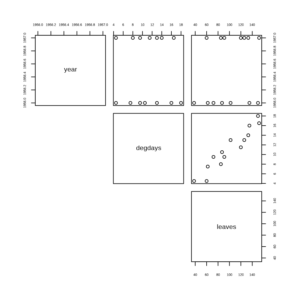
The pairs() function creates a scatterplot matrix of the variables in the dataset. The plot shows the relationships between the variables, including the count of leaves, the number of plants, and the time of observation. The scatterplot matrix helps visualize the relationships between the variables and identify any patterns or trends in the data.
# Fit a Poisson regression model using the glm() function
pois.glm = glm(leaves ~ year + degdays, data=count.data, family=c("poisson"))
# Fit a Poisson regression model using the gam() function
pois.gam = gam(leaves ~ year + s(degdays), data=count.data, family=c("poisson"))
To compare the model we can again use AIC or anova:
anova(pois.glm, pois.gam)Analysis of Deviance Table
Model 1: leaves ~ year + degdays
Model 2: leaves ~ year + s(degdays)
Resid. Df Resid. Dev Df Deviance Pr(>Chi)
1 11.000 6.0593
2 10.569 4.8970 0.43106 1.1623 0.1131The anova() function compares the two models using the likelihood ratio test. The output shows the difference in deviance between the two models, the degrees of freedom, and the p-value for the test. In this case, the p-value is more than 0.05, indicating that the glm model is a better fit than the gam model.
For overdispersed data we have the option to use both the quasipoisson and the negative binomial distributions:
# Fit a Quasipoisson regression model using the gam() function
pois.gam.quasi = gam(leaves ~ year + s(degdays), data=count.data, family=c("quasipoisson"))
summary(pois.gam.quasi)
Family: quasipoisson
Link function: log

Formula:
leaves ~ year + s(degdays)

Parametric coefficients:
              Estimate Std. Error t value Pr(>|t|)
(Intercept) -400.60775   69.08499  -5.799 0.000168 ***
year           0.20708    0.03531   5.865 0.000153 ***
---
Signif. codes:  0 '***' 0.001 '**' 0.01 '*' 0.05 '.' 0.1 ' ' 1

Approximate significance of smooth terms:
             edf Ref.df     F p-value
s(degdays) 1.916   2.39 151.7  <2e-16 ***
---
Signif. codes:  0 '***' 0.001 '**' 0.01 '*' 0.05 '.' 0.1 ' ' 1

R-sq.(adj) =   0.97   Deviance explained = 97.6%
GCV = 0.58311 Scale est. = 0.4138 n = 14# Fit a Negative Binomial regression model using the gam() function
pois.gam.nb = gam(leaves ~ year + s(degdays), data=count.data, family=nb())
summary(pois.gam.nb)
Family: Negative Binomial(12781758.257)
Link function: log

Formula:
leaves ~ year + s(degdays)

Parametric coefficients:
              Estimate Std. Error z value Pr(>|z|)
(Intercept) -407.46535  106.35067  -3.831 0.000127 ***
year           0.21059    0.05436   3.874 0.000107 ***
---
Signif. codes:  0 '***' 0.001 '**' 0.01 '*' 0.05 '.' 0.1 ' ' 1

Approximate significance of smooth terms:
             edf Ref.df Chi.sq p-value
s(degdays) 1.509  1.856  155.8  <2e-16 ***
---
Signif. codes:  0 '***' 0.001 '**' 0.01 '*' 0.05 '.' 0.1 ' ' 1

R-sq.(adj) =  0.967   Deviance explained = 97.3%
-REML = 54.995 Scale est. = 1 n = 14In this tutorial, we covered the basics of Generalized Additive Models (GAMs) in R, focusing on their ability to model complex, nonlinear relationships in data. We started with an overview of how GAMs extend traditional linear models by incorporating flexible, smooth effects for each predictor, making them suitable for nonlinear data. We then explored various R packages, including mgcv and gam, which provide user-friendly functions for fitting and evaluating GAMs, visualizing fitted effects, and assessing model diagnostics. To further understand GAM mechanics, we built a GAM from scratch without using external packages. This hands-on experience demonstrated key principles such as using basis functions for smoothing and the model’s additive nature, allowing us to isolate and effectively combine predictors’ effects. We fit GAM with count and binary data, showcasing their versatility in handling different types of data.