Ordered logistic regression is used when the dependent variable is an ordinal outcome—a categorical variable with a precise rank order but not necessarily equidistant. This method estimates each response level’s probability while considering the outcome’s ordered nature. Typical applications include customer satisfaction assessment, academic grading, and income classification. In this tutorial, we will discuss ordered logistic regression, manually fit a model to understand its mechanics, and use the polr() function from the {MASS} package in R to implement the model. We will also examine coefficients, odds ratios, and category thresholds. This tutorial will provide a practical approach to mastering ordinal logistic regression through concepts and hands-on coding.
Overview
Ordinal logistic regression (OLR) is a statistical method used to analyze the relationship between one or more independent variables (predictors) and an ordinal dependent variable. An ordinal variable is a type of categorical variable where the categories have a specific order, but the intervals between the categories are not uniformly measured. This technique is commonly used in social sciences, psychology, and other fields where data is measured on Likert scales (e.g., strongly disagree, disagree, neutral, agree, strongly agree) or in scenarios where outcomes are ordered such as grades (e.g., A, B, C, D, F). OLR allows researchers to understand the impact of independent variables on the likelihood of an outcome falling into a particular category or higher.
In ordinal logistic regression (OLR), the dependent variable is assumed to have three or more ordered categories. The objective is to predict the probability of an observation falling into one of the categories based on the independent variables’ values. OLR is an extension of logistic regression, which is used for binary outcomes, and it is designed to handle multiple ordered outcome categories.
The key difference between ordinal variables and nominal variables (which have no inherent order, like colors or types of fruit) is that ordinal variables convey a rank or order.
Proportional Odds Assumption: The primary assumption in ordinal logistic regression is that the relationship between each pair of outcome groups is the same across all levels of the independent variables. In other words, the odds ratios comparing any two outcome categories are constant across all levels of the predictor variables.
Model Specification:
Let \(Y\) be an ordinal variable with \(K\) categories. Define \(P(Y \leq k)\) as the probability of being in category \(k\) or lower.
The model assumes that each category has a threshold \(\theta_k\) such that:
The model predicts the probability of \(Y\) falling within each category by computing \(P(Y \leq k)\) for each \(k\).
Interpretation:
The coefficients \(\beta\) represent the change in the log-odds of being in a higher vs. lower category for a one-unit increase in \(X\).
Ordinal Model from Scratch
Fitting an ordinal logistic regression model from scratch in R without using any external packages involves several steps, including creating synthetic data, calculating the cumulative probabilities, estimating the model coefficients using Maximum Likelihood Estimation (MLE), and deriving the summary statistics and odds ratios with confidence intervals. Below, I will outline how to accomplish this step-by-step.
Generate Synthetic Data
We’ll create a synthetic dataset with 6 continuous predictors, one categorical predictor, and an ordinal response variable with three levels.
Code
# Load required package for numerical derivativesif (!require(numDeriv)) install.packages("numDeriv")
Loading required package: numDeriv
Code
# Step 1: Generate Synthetic Dataset.seed(123) # For reproducibilityn <-200# Number of observations# Continuous predictorsX1 <-rnorm(n)X2 <-rnorm(n)X3 <-rnorm(n)X4 <-rnorm(n)# Categorical predictor (two levels)land_type <-sample(c("high land", "medium high land"), n, replace =TRUE)# Convert land_type to a numeric binary variableland_type_numeric <-ifelse(land_type =="high land", 1, 0)# Create a linear predictor and generate response variablelinear_predictor <-1+0.5* X1 -0.3* X2 +0.2* X3 +0.7* land_type_numeric +rnorm(n)# Define thresholds for response categoriesthresholds <-c(-Inf, 0, 1, Inf) # Create three categories (Low, Moderate, High)response <-cut(linear_predictor, breaks = thresholds, labels =c("Low", "Moderate", "High"))# Combine data into a data framedata <-data.frame(X1, X2, X3, X4, land_type_numeric, response)head(data)
# Step 2: Define Model Functions# Function to compute cumulative probabilitiescumulative_probs <-function(X, beta, alpha) { eta <-cbind(1, X) %*% beta # Linear predictor with intercept prob_low <-1/ (1+exp(-(eta - alpha[1]))) prob_moderate <- prob_low / (1+exp(-(eta - alpha[2]))) prob_high <-1- prob_moderatereturn(cbind(prob_low, prob_moderate, prob_high))}# Function to compute the log-likelihoodlog_likelihood <-function(params, data) { beta <- params[1:6] # 8 coefficients for predictors + intercept alpha <- params[7:8] # Two thresholds# Define predictor matrix X (5 predictors plus intercept) X <-as.matrix(data[, c("X1", "X2", "X3", "X4", "land_type_numeric")]) response <-factor(data$response, levels =c("Low", "Moderate", "High"))# Calculate cumulative probabilities probs <-cumulative_probs(X, beta, alpha)# Compute log likelihood ll <-sum(log(ifelse(response =="Low", probs[, 1],ifelse(response =="Moderate", probs[, 2], probs[, 3]))))return(-ll) # Return negative log-likelihood for minimization}
Fit Model
Code
# Step 3: Fit the Model# Function to fit the model using optimfit_model <-function(data) { init_params <-rep(0, 8) # 8 for beta (including intercept) and 2 thresholds result <-optim(init_params, log_likelihood, data = data, method ="BFGS", hessian =TRUE)return(result)}# Fit the modelmodel_fit <-fit_model(data)model_fit$par # Model coefficients (beta) and thresholds (alpha)
# Step 4: Extract Coefficients and Compute Standard Errors# Compute the Hessian matrix and standard errorshessian_matrix <- model_fit$hessianstandard_errors <-sqrt(diag(solve(hessian_matrix)))standard_errors
To evaluate the model’s performance using cross-validation, we’ll use k-fold cross-validation, where we split the data into k folds, train on k-1 folds, and test on the remaining fold. We repeat this process k times, each time using a different fold as the test set, and then compute the average accuracy across all folds.
Code
# Load required package for samplingif (!require(numDeriv)) install.packages("numDeriv")# Function to calculate accuracycalculate_accuracy <-function(true_labels, predicted_labels) {mean(true_labels == predicted_labels)}# Define the model fitting functionfit_model <-function(data) { init_params <-rep(0, 8) # 8 for beta (including intercept) and 2 thresholds result <-optim(init_params, log_likelihood, data = data, method ="BFGS", hessian =TRUE)return(result)}# Define the prediction functionpredict_ordinal <-function(test_data, params) { beta <- params[1:6] # Coefficients for predictors + intercept alpha <- params[7:8] # Thresholds# Define predictor matrix X for test data X <-as.matrix(test_data[, c("X1", "X2", "X3", "X4", "land_type_numeric")])# Compute cumulative probabilities eta <-cbind(1, X) %*% beta # Linear predictor with intercept prob_low <-1/ (1+exp(-(eta - alpha[1]))) prob_moderate <- prob_low / (1+exp(-(eta - alpha[2]))) prob_high <-1- prob_moderate# Combine probabilities into a matrix probs <-cbind(prob_low, prob_moderate, prob_high)# Assign predicted category based on max probability predictions <-apply(probs, 1, function(row) {if (row[1] >= row[2] && row[1] >= row[3]) {"Low" } elseif (row[2] >= row[1] && row[2] >= row[3]) {"Moderate" } else {"High" } })return(predictions)}# Function for k-fold cross-validationk_fold_cv <-function(data, k =5) { n <-nrow(data) fold_size <-floor(n / k) indices <-sample(1:n) accuracies <-c() # Store accuracy for each foldfor (i in1:k) {# Create training and validation sets val_indices <- indices[((i -1) * fold_size +1):(i * fold_size)] train_indices <-setdiff(indices, val_indices) train_data <- data[train_indices, ] val_data <- data[val_indices, ]# Fit the model on the training set fold_fit <-fit_model(train_data)# Predict on validation set val_predictions <-predict_ordinal(val_data, fold_fit$par)# Calculate accuracy for the current fold fold_accuracy <-calculate_accuracy(val_data$response, val_predictions) accuracies <-c(accuracies, fold_accuracy) }# Return the average cross-validation accuracy cv_accuracy <-mean(accuracies)return(cv_accuracy)}# Perform 5-fold cross-validation on the entire datasetset.seed(123)cv_accuracy <-k_fold_cv(data, k =5)print(paste("5-Fold Cross-Validation Accuracy:", round(cv_accuracy *100, 2), "%"))
[1] "5-Fold Cross-Validation Accuracy: 11.5 %"
Fit Ordinal Logistic Regression in R
Fit an ordinal logistic regression model in R using the polr() function from the {MASS} package. We will use the same synthetic dataset created earlier to demonstrate the process. The polr() function fits a proportional odds model to an ordinal response variable using a logistic link function. The model assumes that the coefficients are the same across all levels of the response variable.
Install Required R Packages
Following are the required R packages for this analysis:
Our goal is to develop a Ordinal regression model to predict ordinal class of paddy soil arsenic (non-contaminated, moderately-contaminated and highly-contaminated ) using selected irrigation water and soil properties. We have available data of 263 paired groundwater and paddy soil samples from arsenic contaminated areas in Tala Upazilla, Satkhira district, Bangladesh. This data was utilized in a publication titled “Factors Affecting Paddy Soil Arsenic Concentration in Bangladesh: Prediction and Uncertainty of Geostatistical Risk Mapping” which can be accessed via the this URL
Full data set is available for download can download from my Dropbox or from my Github accounts.
We will use read_csv() function of readr package to import data as a tidy data.
Convert Continuous Variables into Ordinal Variables
An ordinal variable is a type of categorical variable in which the categories have a natural order or hierarchy. Unlike interval or ratio variables, the intervals between the categories are not necessarily equal or measurable. This means that while the categories have a meaningful sequence or ranking, the differences between the categories may not be consistent or quantifiable.
We will convert Soil As (SAs) into three classes:
A. Non-contaminated, SAs < 14.8 mg/kg
B. Moderately-contaminated, SAs 14.8 - 20 mg/kg
C. Highly-contaminated: SAs > 20 mg/kg
Note
14.8 mg/kg is the upper baseline soil arsenic concentration for Bangladesh (Ahmed et al, 2011)
20 mg/kg is the permissible limits of arsenic in agricultural soil [(A Heikens, 2006)](https://agris.fao.org/search/en/providers/122621/records/6472474853aa8c8963049da
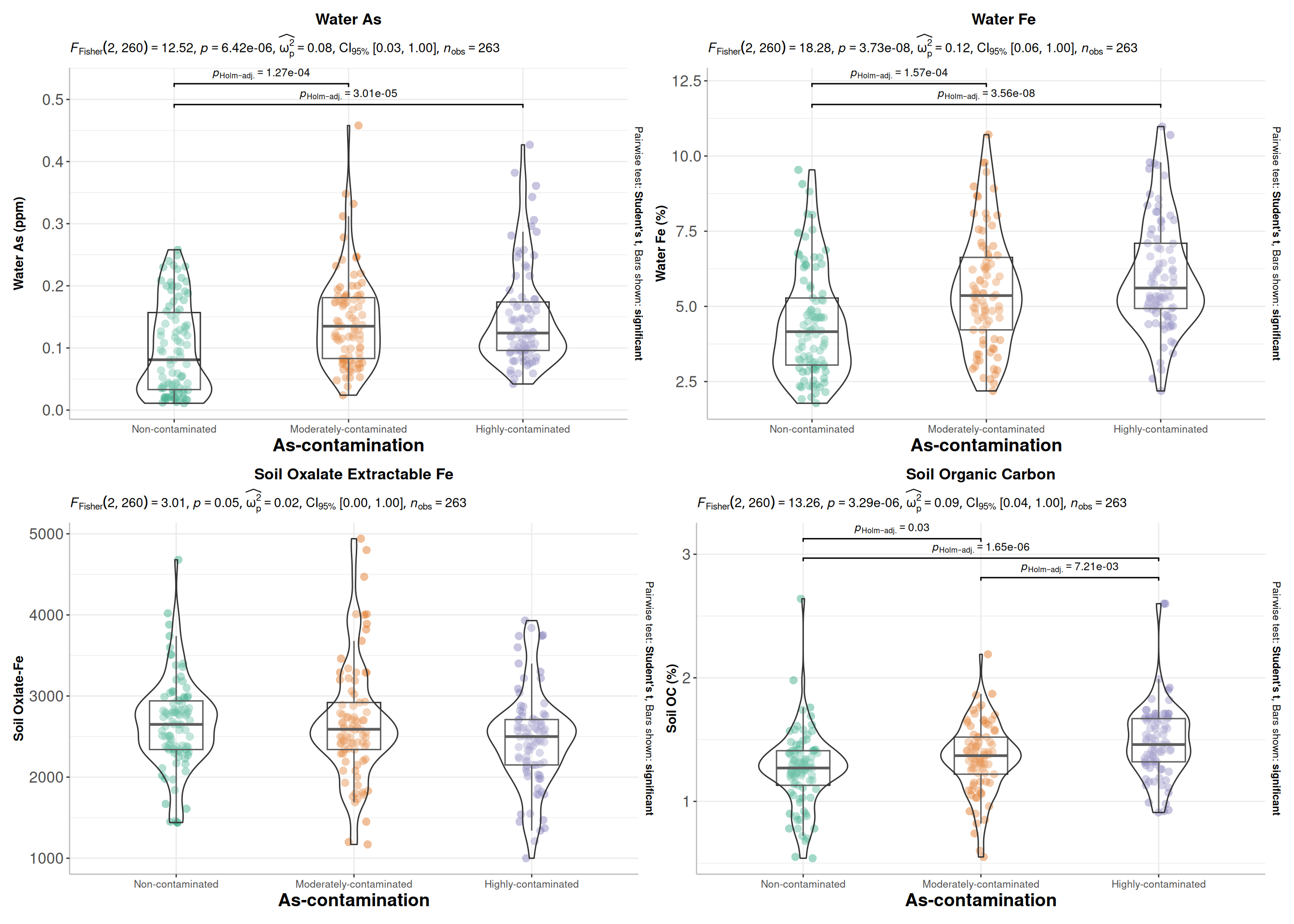
We can create a nice looking plots with results of ANOVA and post-hoc tests on the same plot (directly on the boxplots). We will use gbetweenstats() function of ggstatsplot package:
Code
p1<-ggstatsplot::ggbetweenstats(data = mf,x = Class_As,y = WAs,ylab ="Water As (ppm)",xlab ="As-contamination",type ="parametric", # ANOVA or Kruskal-Wallisvar.equal =TRUE, # ANOVA or Welch ANOVAplot.type ="box",pairwise.comparisons =TRUE,pairwise.display ="significant",centrality.plotting =FALSE,bf.message =FALSE)+# add plot titleggtitle("Water As") +theme(# center the plot titleplot.title =element_text(hjust =0.5),axis.line =element_line(colour ="gray"),# axis title font sizeaxis.title.x =element_text(size =14), # X and axis font sizeaxis.text.y=element_text(size=12,vjust =0.5, hjust=0.5),axis.text.x =element_text(size=8))p2<-ggstatsplot::ggbetweenstats(data = mf,x = Class_As,y = WFe,ylab ="Water Fe (%)",xlab ="As-contamination",type ="parametric", # ANOVA or Kruskal-Wallisvar.equal =TRUE, # ANOVA or Welch ANOVAplot.type ="box",pairwise.comparisons =TRUE,pairwise.display ="significant",centrality.plotting =FALSE,bf.message =FALSE)+# add plot titleggtitle(" Water Fe") +theme(# center the plot titleplot.title =element_text(hjust =0.5),axis.line =element_line(colour ="gray"),# axis title font sizeaxis.title.x =element_text(size =14), # X and axis font sizeaxis.text.y=element_text(size=12,vjust =0.5, hjust=0.5),axis.text.x =element_text(size=8))p3<-ggstatsplot::ggbetweenstats(data = mf,x = Class_As,y = SAoFe,ylab ="Soil Oxlate-Fe",xlab ="As-contamination",type ="parametric", # ANOVA or Kruskal-Wallisvar.equal =TRUE, # ANOVA or Welch ANOVAplot.type ="box",pairwise.comparisons =TRUE,pairwise.display ="significant",centrality.plotting =FALSE,bf.message =FALSE)+# add plot titleggtitle("Soil Oxalate Extractable Fe") +theme(# center the plot titleplot.title =element_text(hjust =0.5),axis.line =element_line(colour ="gray"),# axis title font sizeaxis.title.x =element_text(size =14), # X and axis font sizeaxis.text.y=element_text(size=12,vjust =0.5, hjust=0.5),axis.text.x =element_text(size=8))p4<-ggstatsplot::ggbetweenstats(data = mf,x = Class_As,y = SOC,ylab ="Soil OC (%)",xlab ="As-contamination",type ="parametric", # ANOVA or Kruskal-Wallisvar.equal =TRUE, # ANOVA or Welch ANOVAplot.type ="box",pairwise.comparisons =TRUE,pairwise.display ="significant",centrality.plotting =FALSE,bf.message =FALSE)+# add plot titleggtitle("Soil Organic Carbon") +theme(# center the plot titleplot.title =element_text(hjust =0.5),axis.line =element_line(colour ="gray"),# axis title font sizeaxis.title.x =element_text(size =14), # X and axis font sizeaxis.text.y=element_text(size=12,vjust =0.5, hjust=0.5),axis.text.x =element_text(size=8))
Code
(p1|p2)/(p3|p4)
Data Processing
Code
df <- mf |># select variables dplyr::select (WAs, WFe, SOC, SAoFe, Year_Irrigation, Distance_STW, Land_type, Class_As) |># convert to factor dplyr::mutate_at(vars(Land_type), funs(factor)) |> dplyr::mutate_at(vars(Class_As), funs(factor)) |># normalize the all numerical features dplyr::mutate_at(1:6, funs((.-min(.))/max(.-min(.)))) |>glimpse()
We’ll use the polr() function from the {MASS} package to fit the model. Include the Hess=TRUE option to speed up subsequent calls to summary().
Only Intercept model
Code
# Fit the ordinal logistic regression modelinter.ordinal<-MASS::polr(Class_As~1, data= train,Hess =TRUE)summary(inter.ordinal)
Call:
MASS::polr(formula = Class_As ~ 1, data = train, Hess = TRUE)

No coefficients

Intercepts:
                                            Value   Std. Error t value
Non-contaminated|Moderately-contaminated    -0.5878  0.1547    -3.7996
Moderately-contaminated|Highly-contaminated  0.7346  0.1584     4.6390

Residual Deviance: 399.4273
AIC: 403.4273
Full Model
Code
# Fit the ordinal logistic regression modelfit.ordinal<-MASS::polr(Class_As~., data= train,Hess =TRUE)summary(fit.ordinal)
Call:
MASS::polr(formula = Class_As ~ ., data = train, Hess = TRUE)

Coefficients:
                  Value Std. Error t value
WAs              3.6698     1.1037  3.3249
WFe              2.2060     0.7827  2.8185
SOC              1.6400     1.3379  1.2258
SAoFe           -0.6631     1.0238 -0.6477
Year_Irrigation  4.7694     0.8589  5.5532
Distance_STW    -3.5255     1.2632 -2.7909
Land_typeMHL     1.3473     0.3650  3.6909

Intercepts:
                                            Value   Std. Error t value
Non-contaminated|Moderately-contaminated     2.8381  0.7917     3.5847
Moderately-contaminated|Highly-contaminated  5.0791  0.8642     5.8771

Residual Deviance: 284.2497
AIC: 302.2497
Check the Overall Model Fit
Code
anova(inter.ordinal,fit.ordinal)
Likelihood ratio tests of ordinal regression models

Response: Class_As
                                                                 Model
1                                                                    1
2 WAs + WFe + SOC + SAoFe + Year_Irrigation + Distance_STW + Land_type
  Resid. df Resid. Dev   Test    Df LR stat. Pr(Chi)
1       180   399.4273
2       173   284.2497 1 vs 2     7 115.1776       0
From the above output, you see that the chi-square is 284.2497 and p = <0.0001. This means that you can reject the null hypothesis that the model without predictors is as good as the model with the predictors
Goodness of Fit Tests
The Lipsitz goodness-of-fit test is a statistical tool used to determine how well a logistic regression model predicts binary outcomes. It checks if the observed frequencies of the outcome variable in the sample align with the expected frequencies predicted by the logistic regression model.
Code
generalhoslem::lipsitz.test(fit.ordinal)
    Lipsitz goodness of fit test for ordinal response models

data:  formula:  Class_As ~ WAs + WFe + SOC + SAoFe + Year_Irrigation + Distance_STW + formula:      Land_type
LR statistic = 17.772, df = 9, p-value = 0.03792
Calculate p-values
In a summary output or an ordinal model, p-values are not provided. One way to calculate a p-values is by comparing the t-value against the standard normal distribution, similar to a z test. However, this is only accurate with infinite degrees of freedom, but it can be reasonably approximated by large samples. The accuracy decreases as the sample size decreases.
## calculate and store p valuesp <-pnorm(abs(ctable[, "t value"]), lower.tail =FALSE) *2## combined tablectable <-cbind(ctable, "p value"= p)ctable
                                                 Value Std. Error    t value
WAs                                          3.6697587  1.1037204  3.3248987
WFe                                          2.2059640  0.7826794  2.8184772
SOC                                          1.6399837  1.3378986  1.2257908
SAoFe                                       -0.6631162  1.0237922 -0.6477059
Year_Irrigation                              4.7694354  0.8588574  5.5532329
Distance_STW                                -3.5254761  1.2632236 -2.7908568
Land_typeMHL                                 1.3472678  0.3650260  3.6908817
Non-contaminated|Moderately-contaminated     2.8380559  0.7917057  3.5847361
Moderately-contaminated|Highly-contaminated  5.0790576  0.8642141  5.8770827
p value
WAs 8.845065e-04
WFe 4.825204e-03
SOC 2.202774e-01
SAoFe 5.171752e-01
Year_Irrigation 2.804340e-08
Distance_STW 5.256873e-03
Land_typeMHL 2.234780e-04
Non-contaminated|Moderately-contaminated 3.374192e-04
Moderately-contaminated|Highly-contaminated 4.175597e-09
Confidence Intervals
We can calculate confidence intervals for the parameter estimates using two methods: profiling the likelihood function or using standard errors and assuming a normal distribution. It’s important to note that profiled confidence intervals are not always symmetric, although they are typically close to being symmetric. If the 95% confidence interval does not include 0, the parameter estimate is considered statistically significant.
The coefficients in the model can be hard to understand because they are scaled in logs. Another way to interpret logistic regression models is to change the coefficients into odds ratios. To find the odds ratio and confidence intervals, we just need to raise the estimates and confidence intervals to the power of the mathematical constant e.
The tbl_regression() function from the gtsummary package takes a regression model object as input and produces a formatted table with Odd-ratio and confidence interval.
Code
tbl_regression(fit.ordinal, exp =TRUE)
Characteristic
OR
95% CI
WAs
39.2
4.79, 368
WFe
9.08
2.00, 43.5
SOC
5.16
0.38, 74.9
SAoFe
0.52
0.07, 3.84
Year_Irrigation
118
23.1, 677
Distance_STW
0.03
0.00, 0.32
Land_type
HL
—
—
MHL
3.85
1.89, 7.95
Abbreviations: CI = Confidence Interval, OR = Odds Ratio
The tab_model() function of {sjPlot} package also creates HTML tables from regression models:
Code
tab_model(fit.ordinal)
Class_As
Predictors
Odds Ratios
CI
p
Non-contaminated|Moderately-contaminated
17.08
3.58 – 81.51
<0.001
Moderately-contaminated|Highly-contaminated
160.62
29.17 – 884.32
<0.001
WAs
39.24
4.79 – 367.93
0.001
WFe
9.08
2.00 – 43.48
0.005
SOC
5.16
0.38 – 74.85
0.222
SAoFe
0.52
0.07 – 3.84
0.518
Year Irrigation
117.85
23.12 – 676.76
<0.001
Distance STW
0.03
0.00 – 0.32
0.006
Land type [MHL]
3.85
1.89 – 7.95
<0.001
Observations
182
R2 Nagelkerke
0.528
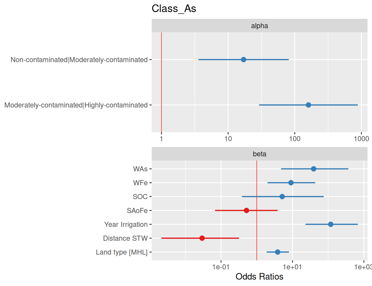
plot_model() function of {sjPlot} package creates plots the estimates from logistic model:
Code
plot_model(fit.ordinal, vline.color ="red")
In the summary output, you’ll see coefficients for each predictor variable, along with their standard errors and z-values. These coefficients represent the log odds ratios.
Interpret the Odds Ratios
Exponentiate the coefficient: This converts the log odds ratio to an odds ratio. For example, if the coefficient for WAs is 8.195, the odds ratio associated with a one-unit increase in WAs is \(e^{8.195}\)
Interpret the odds ratio: When the odds ratio is greater than 1, it means that for each one-unit increase in the predictor variable, the odds of being in a higher category of the outcome increase by the value of the odds ratio. On the other hand, if the odds ratio is less than 1, it indicates that for each one-unit increase in the predictor variable, the odds of being in a higher category of the outcome decrease by the reciprocal of the odds ratio.
Check the significance: When interpreting the results, it’s important to pay attention to the p-values associated with each coefficient. A p-value that is less than 0.05 suggests that the odds ratio is significantly different from 1, indicating a strong association between the predictor variable and the outcome category. It’s crucial to remember that interpretation should always be done in the context of the specific research question and the nature of the data being analyzed.
Model Performance
Code
performance::performance(fit.ordinal)
Can't calculate log-loss.
# Indices of model performance

AIC     |    AICc |     BIC | Nagelkerke's R2 |  RMSE | Sigma
-------------------------------------------------------------
302.250 | 303.296 | 331.086 |           0.528 | 1.848 | 1.274
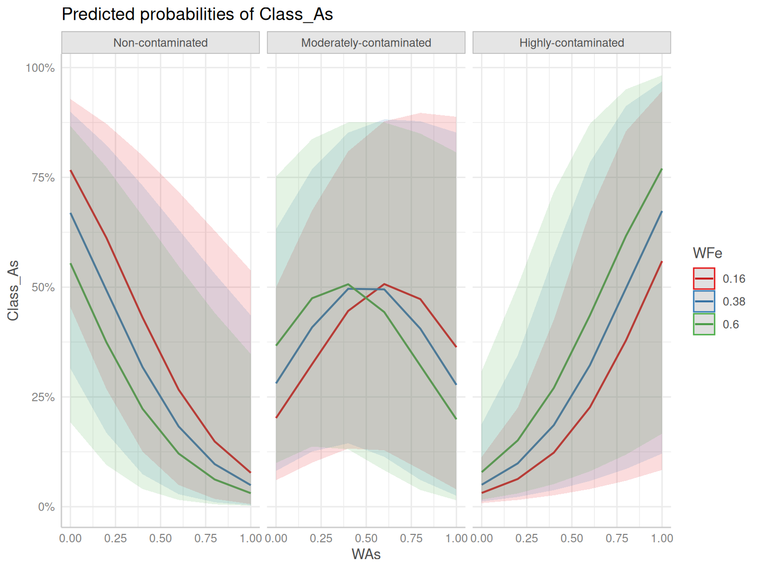
ggeffects supports labelled data and the plot()- method automatically sets titles, axis - and legend-labels depending on the value and variable labels of the data.
# Set the number of foldsK <-5# Create a vector to store misclassification rates for each foldmisclassification_rates <-numeric(K)# Set seed for reproducibilityset.seed(123)# Generate fold indicesfolds <-sample(rep(1:K, length.out =nrow(df)))# Loop through each foldfor (k in1:K) {# Split the data into training and test sets train_data <- df[folds != k, ] test_data <- df[folds == k, ]# Fit the model on the training data model<-MASS::polr(Class_As~., data= df,Hess =TRUE)# Predict the class labels on the test set predicted_classes <-predict(model, newdata = test_data, type ="class")# Calculate the misclassification rate for the current fold misclassified <-mean(predicted_classes == test_data$Class_As) fold_misclassification_rate <- misclassified /nrow(test_data)# Store the misclassification rate for this fold misclassification_rates[k] <- fold_misclassification_rate}# Calculate the average misclassification rate across all foldsavg_misclassification_rate <-mean(misclassification_rates)# Display resultscat("Cross-Validated Misclassification Rates for Each Fold:", misclassification_rates, "\n")
Cross-Validated Misclassification Rates for Each Fold: 0.01281595 0.01174795 0.01317195 0.01368343 0.008505917
Understanding ordinal regression and how to implement it in R can provide valuable insights into the relationships between predictor variables and ordinal response variables. This can lead to a deeper understanding of the factors influencing the outcome of interest. It’s important to approach ordinal regression carefully, taking into consideration the specific data and research question.