1. Linear Quantile Regression

Linear Quantile Regression (LQR) is a statistical method that models the relationship between predictor variables and specific quantiles (e.g., median, 90th percentile) of the response variable. Unlike Ordinary Least Squares (OLS) regression, which estimates the conditional mean of the response variable, quantile regression provides a more complete picture by estimating conditional quantiles. This makes it robust to outliers and useful for analyzing non-normal or heteroscedastic data.

Key Concepts

(1) Quantiles vs. Mean

  • Mean (OLS Regression): Minimizes the sum of squared residuals → sensitive to outliers.

  • Quantiles (Quantile Regression): Minimizes the sum of asymmetrically weighted absolute residuals → robust to outliers.

(2) Conditional Quantile Function

  • For a given quantile τ ∈ (0,1) (e.g., τ = 0.5 for the median), the model estimates:

\[ Q_{Y|X}(\tau) = X \beta(\tau) \]

where:

  • \(Q_{Y|X}(\tau)\) = τ-th quantile of \(Y\) given predictors \(X\).

  • \(\beta(\tau)\) = regression coefficients for quantile τ.

(3) Loss Function

Quantile regression minimizes:

\[ \sum_{i=1}^{n} \rho_{\tau}(y_i - X_i \beta(\tau)) \]

where: \[ \rho_{\tau}(u) = \begin{cases} \tau u & \text{if } u \geq 0 \\ (\tau - 1)u & \text{if } u < 0 \end{cases} \] - This asymmetrically weights residuals depending on whether they are above or below the quantile.

Advantages Over OLS Regression

Feature OLS Regression Quantile Regression
Estimates Conditional mean Conditional quantiles (median, 90th percentile, etc.)
Robustness Sensitive to outliers Resistant to outliers
Heteroscedasticity Assumes constant variance Works with varying variance
Distributional Insight Only models the mean Models entire conditional distribution

When to Use Linear Quantile Regression?

Skewed Data (e.g., income, medical costs)
Heteroscedasticity (variance changes with predictors)
Outliers Present (OLS can be misleading)
Interest in Extremes (e.g., 90th percentile risk analysis)

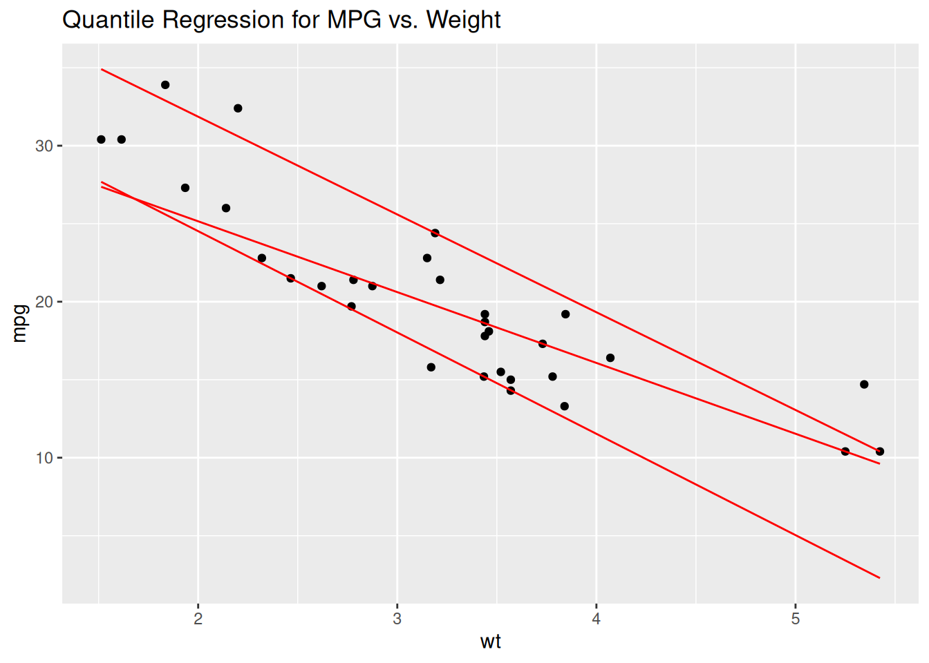
Quantile Regression in R

Using the quantreg Package

Code
#install.packages("quantreg")
library(quantreg)
Loading required package: SparseM
Code
# Fit median regression (τ = 0.5)
model <- rq(mpg ~ wt + hp, data = mtcars, tau = 0.5)
summary(model)

Call: rq(formula = mpg ~ wt + hp, tau = 0.5, data = mtcars)

tau: [1] 0.5

Coefficients:
            coefficients lower bd upper bd
(Intercept) 36.62601     31.41282 38.90949
wt          -3.60570     -5.91208 -2.81272
hp          -0.03559     -0.04981 -0.01885
Code
# Fit multiple quantiles (τ = 0.1, 0.5, 0.9)
model_multi <- rq(mpg ~ wt + hp, data = mtcars, tau = c(0.1, 0.5, 0.9))
summary(model_multi)

Call: rq(formula = mpg ~ wt + hp, tau = c(0.1, 0.5, 0.9), data = mtcars)

tau: [1] 0.1

Coefficients:
            coefficients lower bd upper bd
(Intercept) 34.00732     24.65673 41.82161
wt          -4.47409     -8.31500 -0.60609
hp          -0.01524     -0.10200 -0.01051

Call: rq(formula = mpg ~ wt + hp, tau = c(0.1, 0.5, 0.9), data = mtcars)

tau: [1] 0.5

Coefficients:
            coefficients lower bd upper bd
(Intercept) 36.62601     31.41282 38.90949
wt          -3.60570     -5.91208 -2.81272
hp          -0.03559     -0.04981 -0.01885

Call: rq(formula = mpg ~ wt + hp, tau = c(0.1, 0.5, 0.9), data = mtcars)

tau: [1] 0.9

Coefficients:
            coefficients lower bd upper bd
(Intercept) 42.39191     39.07599 45.68323
wt          -3.07037     -5.86784 -2.84869
hp          -0.04905     -0.06179  0.07345

Visualizing Quantile Regression

Code
library(ggplot2)
ggplot(mtcars, aes(x = wt, y = mpg)) +
  geom_point() +
  geom_quantile(quantiles = c(0.1, 0.5, 0.9), color = "red") +
  labs(title = "Quantile Regression for MPG vs. Weight")
Smoothing formula not specified. Using: y ~ x

Interpreting Output

  • Coefficients show how predictors affect different quantiles.
  • Example: If β(wt) for τ=0.9 is more negative than for τ=0.1, heavier cars have a stronger negative effect on high MPG values.

Extensions of Quantile Regression

  1. Nonlinear Quantile Regression (using splines or neural networks).
  2. Bayesian Quantile Regression (for uncertainty quantification).
  3. Censored Quantile Regression (for survival data).
  4. High-Dimensional Quantile Regression (with LASSO/ridge penalties).

Conclusion

Linear Quantile Regression is a powerful alternative to OLS when: - You care about different parts of the distribution (not just the mean). - Your data has outliers, skewness, or heteroscedasticity. - You need robust estimates for decision-making (e.g., risk analysis).

By estimating conditional quantiles, it provides deeper insights into how predictors influence the entire distribution of the response variable.